Multi-Fractal Analysis of Daily Air Temperature Time Series in Coastal Areas of China

With the intensification of global warming, extreme temperature events have become more and more frequent, resulting in serious damage to the ecological environment, societies, economies, and human health (Sun et al. ^[1]; Leeson et al. ^[2]; Sheridan and Lee ^[3]). Studies have confirmed that the disastrous events caused by extreme temperatures, particularly typhoons, heat weaves, cold waves, droughts and so on, have become more frequent in China (Chen et al. ^[4]; Liu et al. ^[5]; Yue et al. ^[6]), and have taken a heavy toll on the Chinese economy (Cui et al. ^[7]; Wang and Zablon ^[8]). China has a sensitive and vulnerable climate, which is obviously affected by climate warming. Therefore, it is urgent to understand the way in which regional temperature changes and its regulation mechanism.

As one of the most important elements in the climate system, air temperature is characterized by its uncertainty and spatio-temporal heterogeneity (Tang et al.^[9]; Tang et al.^[10]; Hanna et al.^[11]), which is synthetically influenced by solar radiation, atmospheric circulation, land-sea thermal properties difference, topography, vegetation and many other factors. It is impossible to describe the inherent regulation mechanism and its nonlinear characteristics of climate system with just one single fractal dimension. Furthermore, the traditional methods for studying randomness and determinacy have some insurmountable defects in exploring the long-term evolution behavior of nonlinear systems, and therefore they all fail to remove the interference signals from the original temperature time series. Besides, the different independence test methods used to identify the short-range correlation often fail to identify the time series with long-range correlation (He et al.^[12]; Wang et al.^[13]; Herrera-Grimaldi et al.^[14]). The Detrended Fluctuation Analysis (DFA) method can help to identify the multifractal strength of internal fluctuations and the long-range correlation (LRC) in the evolution process of temperature time series, but this method cannot characterize long-range related non-stationary time series and describe the multiscale fractal subsets (Karatasou and Santamouris^[15]; Mali^[16]). In 2002, Kantelhardt et al. ^[17] proposed the Multi-fractal Detrended Fluctuation Analysis (MF-DFA) method for investigating the multifractal characteristics of temperature time series. Since then, the MF-DFA method has been used to describe the fluctuation distribution of different local conditions affecting the whole series and to analyze the effect of influencing factors on small fluctuations. At present, the MF-DFA method has been widely used in different fields (Kantelhardt et al.^[17]; Kalamaras et al.^[18]; Pedron^[19]; Du et al.^[20]; Cabrera-Brito et al.^[21]; Zhang et al.^[22]; Subhakar and Chandrasekhar^[23]), such as atmosphere science, marine science, and financial market analysis.

The temperature variation changes with latitude and altitude (Chakraborty et al.^[24]; Lee et al.^[25]). China has a vast territory, with multiple temperature zones and a diverse climate. The climate in the north and the south are distinctively different. In the recent 60 years, the average temperature rise rate of some regions in north China and the Qinghai-Tibet Plateau is several times higher than that of other places in China. However, compared with the distinct long-term warming trend in east China, the rise of air temperature in southwest China is not obvious (Zeng et al.^[26]; Wu et al.^[27]). As for the climate system itself, it has characteristics of long-range power-law correlations and long persistence (Li et al.^[28]; Yuan et al.^[29]; Cleveland et al.^[30]; He and Zhao^[31]). The intrinsic LRC have shown that the spatio-temporal fluctuation of temperature series is not only caused by external random disturbances, but also caused by its inherent complex nonlinear correlations that come from the cumulative effect in the process of temperature formation and evolution, namely the"multifractality". Once there are certain differences in certain types of behavior at different periods, multifractality may arise, given similarities between different types of temperature evolution behavior.

Multifractality can be used to identify the internal stability of climate systems, distinguish the strength of self-regulation mechanism of the system, and explore how the internal long-range correlation of time series evolves. These system properties are critical to the analysis of temperature changes. However, the above laws and their characteristics cannot be analyzed by traditional methods. A number of domestic and overseas scholars have examined the characteristics of spatio-temporal air temperature change and estimated their influence on the environment (Zhong et al.^[32]; Zhu et al.^[33]; Kalamaras et al.^[34]), and a few have investigated the internal causes of temperature change. However, few scholars are known for the analysis of the difference between temperature change and its triggering mechanism in different temperature zones of monsoon climate, which is of great significance for a better understanding of climate change and its evolution. As a region with the largest population density and the highest level of economic development, the coastal region of east China, whose response to and risk of global warming are highly complex and uncertain, cannot be ignored in its sensitivity to temperature warming, and therefore it is extremely necessary to carry out researches about this region. In the present research, the typical temperature zones of the eastern coastal regions in Guangdong, Jiangsu and Liaoning Provinces are chosen for research as they cover the tropics, subtropics and temperate regions. The MF-DFA method has been adopted to study the internal driving mechanism of temperature change in various regions and to analyze the multifractal characteristics, which can help deepen the understanding of how temperature changes and its causes in different temperature zones in China under the background of climate change, and provide theoretical reference and scientific guidance for our response to regional climate change.

The structure of this paper is as follows. After the data sources and methods are briefly described (section 2), the MF-DFA results of T_avg, T_max, and T_min which mainly have multifractal strength and long-range correlation are analyzed in section 3. Based on this, the discussion is given in section 4. The multifractal behaviors of temperature time series (section 4.1) and the causes of LRC (section 4.2) are discussed, and the characteristics of fluctuations of temperature time series (section 4.3) are analyzed. Conclusions are provided in section 5.

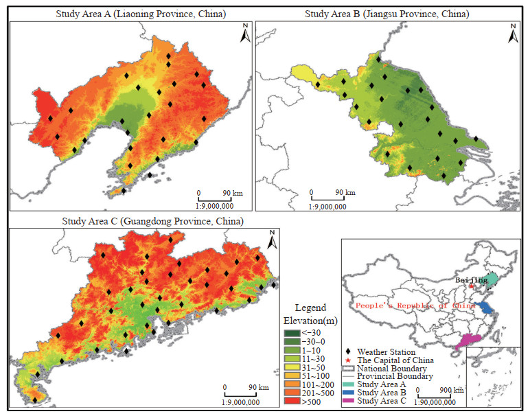
As a southern province of China, Guangdong has a tropical and subtropical monsoon climate. Therefore, it has long summers and warm winters. The average annual temperature is from 20.4 ℃ to 23.1 ℃. Jiangsu is an eastern-central province of China and is situated in a transitional area between temperate and subtropical zone. Generally, the south of the Huaihe River and sub-northern irrigation canal is a humid subtropical climate zone, whereas the north of the Huaihe River is a warm temperate climate zone. Its annual average temperature is from 13 ℃ to 16 ℃, increasing from northeast to southeast. Liaoning is a northern coastal province in northeast China and is located in temperate monsoon climate zone. The temperature in this area is characterized by uneven spatial distributions, decreasing from the plain to the mountainous area. The annual average temperature in Liaoning is from 7 ℃ to 11 ℃.

The daily temperature records from January 1, 1980 to December 31, 2017 for the three provinces were collected from 90 meteorological stations of the China Meteorological Administration (https://data.cma.cn/site/index.html). The stations were selected on the basis of the length of the time series, data completeness (missing values less than 5%), and spatial coverage. A series of quality control tests were applied to identify outliers at all stations and all the outliers were marked with a quality control flag. The maximum, average, and minimum daily temperatures were then extracted. It should be noted that the level of data completeness in the study exceeded the minimum requirement of 95%. At this level, scaling indices and scaling behaviors of the time series were not affected (Durre et al.^[35]).

Figure 1.  Location and digital elevation model of the study areas.

When the temperature time series is analyzed by using Fourier transform, the periodic fluctuation of temperature time series may lead to crossover (Li et al.^[28]; Yuan et al.^[29]). Therefore, periodical components of temperature time series were removed by employing the Seasonal and Trend decomposition using the Loess (STL) method (Cleveland et al.^[30]).

Generally, the temperature series are affected by noise and non-stationary signals. The potential trend components in the signals caused by internal long-range fluctuations can interfere with the recognition of the multifractal strength and the LRC of the series, which will therefore result in a failure to reveal how the temperature system evolves in the complex environment. The traditional research methods have ignored the short-term potential trend components that exist in the temperature series, and have therefore failed to eliminate the interference of local trend to the long-range correlation analysis. However, the MF-DFA method can remove the interference of various kinds of noise to the system, thus avoiding the false detection of short-range correlation and non-stationary time series as long-range correlation, which solves the problem that the traditional stochastic and deterministic methods have insurmountable defects in exploring the long-term behavior of nonlinear systems.

The MF-DFA method can remove the interference of various kinds of noise to the time series and correctly identify the long-range correlation within the system. However, it also eliminates the short-term trend fluctuations and periodic signals in the series, and therefore fails to identify the short-term correlation of the system. For the research on the periodic variation law of each natural system, such as year, season, month, day, etc, the methods of Fourier transform, maximum entropy spectrum analysis and wavelet analysis are obviously better than the MF-DFA method. The MF-DFA is an effective tool for measuring the multifractal data of temperature time series. For more details of this method, please refer to Jiang et al.^[36].

(1) The accumulated deviation computation of time series. For a given time series x_i (i=1, 2, 3, ..., N), establish the cumulative deviation series y:

In the formula, x is the mean value of the original series.

(2) The y series is divided into the non-overlapping subintervals with the equal length s, and the number of subintervals N_s can be expressed as N_s = int(N/s). Because N_s is not necessarily divisible by s, the y series will be divided again from its tail in reverse order so as to ensure the integrity of the information, thus obtaining 2 N_s subintervals.

(3) For each v subinterval, the least square method is used to fit the k-order polynomial, and the local trend function is thereby obtained:

In the formula, a_k is the fitting polynomial coefficient, and k is the highest order of the polynomial.

(4) By eliminating the trend in each sub-interval, namely, the cumulative deviation minus the trend function, the mean value of its variance can be obtained:

The local detrend fluctuation function F(v, s) can be obtained by calculating the square root of formula (3), while the function F(v, s) can be obtained by calculating the square root for the mean value of variance over the entire divided data intervals:

(5) Calculate the q-order detrend fluctuation function of the whole series:

In the formula, q can be any non-zero real number. When q is equal to zero, the fluctuation function is:

(6) Taking the logarithmic operation for F_q(s), we can obtain the relation of the log-log coordinate graph F_q (s) s^H(q), where H(q) is the scaling exponent of the fluctuation function, so there is

(7) Then the formula (7) can be rewritten as follows:

(8) Take logarithm on both sides:

In the formula, H(q) denotes the generalized Hurst exponent. When q is equal to two, H(2) is the Hurst exponent H, and its numerical value represents the strength of long-range correlation of the original series. When H is less than 0.5, the series has a negative longrange correlation, and the current trend of the series is opposite to its future trend; that is to say, if the current trend is decreasing (or increasing), then the future trend will be increasing (or decreasing). When H is equal to 0.5, the series is irrelevant; that is, there is no relation between the current and future trends of the series. When H is less than or equal to one and greater than 0.5, the series has a long-range correlation, indicating that the current trend is the same as the future trend; that is to say, if the current trend is decreasing (or increasing), then the future trend will be decreasing (or increasing). And the greater the H is, the stronger the correlation will become.

The fluctuation function F_q(s) is also affected by the q-value. When q < 0, F_q(s) is mainly dominated by small fluctuations; when q > 0, F_q(s) is mainly influenced by large fluctuations. When H(q) changes with q, this indicates that the original series has varying degrees of fluctuation; that is, the original series has multifractal characteristics. When H(q) remains unchanged, the original series has no multifractal characteristics.

In addition to the generalized Hurst exponent method, there are methods of mass exponent τ(q), singularity exponent α, and multifractal spectrum f (α) that describe the multifractal characteristics of time series, and their transformation relations are as follows:

The width Δα of the multifractal spectrum f(α) can measure the strength of the multifractal characteristics; that is, the larger Δα is, the stronger the multifractal characteristics become.

In the article, random sequences are acquired based on an original data series by using shuffled and surrogate random number generation algorithms. Use of the algorithm Fisher-Yates random shuffle can generate shuffled data (Durstenfeld^[37]; Lemire^[38]), and the Fisher-Yates random shuffle described by Knuth requires one random integer in an interval for each value in an array to be shuffled. The random permutations generated by this algorithm are equiprobable and at the same time this algorithm is efficient.

Fisher-Yates random shuffle: it shuffles an array of size n so that n! will possibly permutate. Assuming that array A includes n elements which are subscripts from 0 to n-1, the specific algorithm is as follows.

(1) Write numbers from 1 to n.

(2) Take a random number k from 1 to the remaining numbers (including this number).

(3) Starting from the lower places, obtain k numbers (this number has not been taken out) and write it in the last place of a separate list.

(4) Repeat step 2 until all numbers are taken out.

(5) Obtain a random permutation of the original numbers which is a permutation obtained in step 3.

It has been proved that if the number taken out in step 2 is truly random, then the resulting permutation must be the same,

for i = n - 1, …, 1 do

    j ← random integer in [0, i]

    exchange A[i]and A[j]

end for

Surrogate data are essentially transformations of a time series that preserve some features of the time series but not others. Their main purpose is to test a hypothesis about the structure of the time series such as the randomness of the time series, the nonlinearity of the time series and so on by comparing the measured data to the surrogate.

Iterative amplitude adjusted Fourier transform (IAAFT) surrogates are proposed by Schreiber & Schmitz. They are constructed by iterative replacement of Fourier amplitudes with the correct values and rescaling the distribution to achieve a closer match between both the distribution and the power spectrum in the original data and the surrogates. The power spectrum and amplitude distribution of the original time series should be preserved in the surrogate algorithm. The iterative nature of the IAAFT alternative algorithm will increase the calculation time, which depends on the number of iterations required for convergence. The specific algorithm is as follows.

(1) Generate a random shuffle of the data, y_n⁽⁰⁾

(2) Fourier transform the current iteration y_n⁽ⁱ⁾, replace Fourier amplitudes (but not phases) with those from the original signal and inverse Fourier transform. This generates a signal, z_n⁽ⁱ⁾, which has the same power spectrum as the original time series but a slightly different distribution of values.

(3) Rescale z_n⁽ⁱ⁾ to the original distribution of s_n to produce the next iteration y_n^{(i + 1)} = s_rank(znⁱ)

(4) Repeat steps 2-3 until the exact reordering in step 3 is repeated, i.e. rank (z_n^{(i + 1)}) = rank(z_n⁽ⁱ⁾) for all n. This indicates that the procedure has converged, and that the power spectrum and distribution are as close to the original data as possible.

(5) As for the final surrogate signal, it either takes the last z_n of step 2 to exactly preserve the power spectrum (IAAFT-2), or the last iteration of step 3 to exactly preserve the amplitude distribution (IAAFT-1).

The subtropical zone, the subtropical-warm temperate transition zone and the typical regions of temperate climate zone were selected as representatives to study the regional difference characteristics and their changing trend of daily T_avg, T_max and T_min temperature series in Guangdong, Jiangsu and Liaoning from 1980 to 2017.

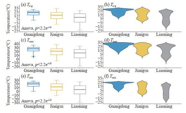
In Fig. 2, all the T_avg, T_max and T_min of the box plots and violin plots indicate that the temperature series had a tendency to decrease with the increase of latitude. According to Fig. 2a, c and e, we know the symmetry of data distribution, the dispersion degree, the outliers and the skewness of data, which showed the position of the series quantile. The T_avg, T_max and T_min of Guangdong, Jiangsu and Liaoning showed significant regional differences between different climatic zones, decreasing from subtropics to temperate zones. The multi-year average fluctuation range of T_avg was the smallest in Guangdong province, followed by Jiangsu province and the largest in Liaoning province, while the median value of T_avg was in the opposite order. And it was also the same for T_max and T_min of the above three provinces. The minimum value of T_avg, T_max and T_min for each province was respectively in the decreasing order of Guangdong, Jiangsu and Liaoning. And the maximum value of temperature for each province was in the decreasing order of Jiangsu, Guangdong, and Liaoning. Fig. 3b, d, and f show the probability density distribution of temperature series and the density of any position. And the probability density distribution patterns of T_avg, T_max and T_min were significantly different. The T_avg, T_max and T_min distributions of Guangdong were relatively concentrated, while the temperature series distribution in Liaoning was relatively dispersed with the largest range. In Guangdong, the probability distributions of T_avg, T_max and T_min were not uniform, and the probability function of all temperature values was relatively high. In Fig. 3, the T_avg of Guangdong was concentrated in the relatively high temperature range from 20 ℃ to 30 ℃, which denoted that Guangdong had the smallest temperature difference. The temperature distribution in Jiangsu was relatively uniform. In Liaoning, its temperature difference was the largest. And the fat-tail distribution of air temperature was more obvious there, which was mainly concentrated in the higher and lower ranges.

Figure 2.  Temperature statistical distribution chart from 1980 to 2017. Box plots for air average temperature (a), maximum temperature (c), and minimum temperature (e) with quartile (box) and maximum/ minimum during the period 1980-2017 of Guangdong (GD), Jiangsu (JS) and Liaoning (LN) Provinces. Violin plots for air average temperature (b), maximum temperature (d), and minimum temperature (f) with data distribution and their probability density for the period 1980-2017 for GD, JS, and LN Provinces.

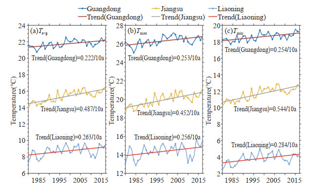
Figure 3.  Annual temperature changes in Guangdong, Jiangsu and Liaoning. Annual average temperature, T_avg (a), maximum temperature, T_max (b), minimum temperature, T_min (c) for Guangdong, Jiangsu and Liaoning for the period from 1980 to 2017.

In Fig. 3 the upward trend in annual average temperature showed that the three provinces were warming during the period from 1980 to 2017. Jiangsu had a higher rate of temperature increase as compared with Liaoning and Guangdong. Furthermore, as observed in Fig. 4, Liaoning had the largest year to year variability for T_avg, T_max, and T_min.

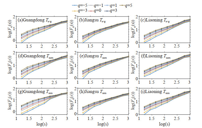
Figure 4.  Log-log plots of the q-order fluctuation function F_q(s) versus time scale s for the different temperature series in Guangdong, Jiangsu and Liaoning. (a)-(c) respectively denotes the average temperature (T_avg) of Guangdong, Jiangsu and Liaoning, (d)-(f) respectively denotes the maximum temperature (T_max) of Guangdong, Jiangsu and Liaoning, and (g)-(i) respectively denotes the minimum temperature (T_min) of Guangdong, Jiangsu and Liaoning.

Based on the MF-DFA method, the author adopted the methods of generalized Hurst exponent H (q), mass exponents τ(q), singularity spectrum f(α) and singularity exponents α to study the multifractal characteristics of T_avg, T_max and T_min in different temperature zones.

Figure 4 shows that the T_avg, T_max and T_min all had good power-law relations, and the air temperature had obvious multifractal characteristics, which indicated that the fluctuation of the internal evolution of temperature series was not random, but was caused by its long-range correlation. For different q values and their corresponding q-order Root-Mean-Square (RMS), the difference between them is more obvious in small scale segmentation than in large scale segmentation. The number of small segments and large segments included in different local periods were different, small segments could distinguish the large and small fluctuations of different local periods. In contrast, large segments spanned multiple local periods with small and large fluctuations, thus averaging the differences of their fluctuation amplitude. With the increase of the number of segmented samples, the q-order RMS of the multifractal time series would also increase, thus resulting in the decrease of the H(q) of the multifractal time series.

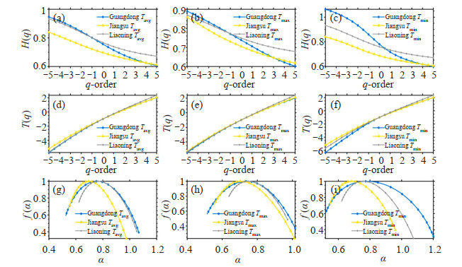
It could be seen from Fig. 5 a-c that, for a given fitting polynomial, the generalized Hurst exponent H(q) of T_avg, T_max and T_min all showed dependence on q, and its nonlinearity decreased with the increase of q, showing a nonlinear feature with homogeneity. The generalized Hurst exponent H (q) varied with q, which revealed the multifractality of the temperature records. For all the cases, H(q) > 0.5 was observed, indicating a long-term positive correlation with the temperature record. And this suggested that a high value of temperature might be observed after another high value of temperature. Furthermore, it was observed that the multifractality was weaker for positive values as the slope of H (q) was larger for negative q values (the small fluctuations) than that of the positive ones (the large fluctuations). This phenomenon indicated that there was a higher degree of multifractality in the smaller fluctuation.

Figure 5.  Multifractal characteristic graphs of T_avg, T_max and T_min in Guangdong, Jiangsu and Liaoning. (a)-(c) shows the curve graph of generalized Hurst exponent H(q) versus q-order; (d)-(f) shows the curve graph of mass exponents τ(q) versus q-order; (g)-(i) shows the singularity spectrum f(α) and singularity exponents α.

It could be seen from Fig. 5 d-f that the mass exponent τ(q) grew with the increase of q, showing an obvious nonlinear relationship of the convex increasing function τ(q). And the temperature time series showed distinctive multifractality. Moreover, the plots indicated that the temperature of Guangdong had the highest degree of multifractality. Moreover, the nonlinear characteristics of temperature series τ(q)~q in Guangdong were more significant than the rest two regions, which denoted that Guangdong had the highest degree of multifractality.

It could be seen from Fig. 5 g-i that the curve shapes of the T_avg, T_min and T_max singularity spectrum were asymmetrical, which denoted the multifractal characteristics of temperature time series. Moreover, the spectrum had a left truncation and a long right tail, which indicated that the temperature time series had the multifractal structures with many small fluctuations that were insensitive to local fluctuations with large magnitudes. The results showed that the small fluctuations dominated the temperature time series, which was one of the important reasons for the time series to have long-range correlations. These fluctuations also reflected the internal dynamic features within the temperature time series. The structure of the multifractal spectrum was almost similar for all temperature time series, indicating a similar evolution pattern.

In order to measure the multifractal strength of all the temperature time series data in the research areas, the author calculated ΔH (q), Δα, Δf and H(2) respectively. The H(2) of the T_avg, T_min and T_max time series respectively was the highest for Liaoning, followed by Guangdong and Jiangsu. All the Hurst exponents H(2) were greater than 0.5, which indicated that the multifractality of these temperature time series represented positive LRC. Furthermore, the LRC followed the same order, which meant that an increase or decrease was likely to be followed by another increase or decrease in temperature. The ΔH (q) and Δα for all temperature time series were the largest for Guangdong, revealing the highest degree of multifractality. Both ΔH (q) and Δα for the T_avg and T_min time series for Jiangsu were smaller than that of Liaoning, while for the T_max, both ΔH (q) and Δα for Jiangsu were larger than that of Liaoning. The multifractal spectrum width Δα reflected the multifractality degree, which could reveal the probability distributions of the fluctuations. The larger Δα, the stronger the multifractality degree and the more complex the multifractal structure of the temperature time series. In all these cases, each Δf was greater than zero, indicating that the probability of high level fluctuations in temperature was dominant. Meanwhile, there was a distinct internal change in the time series, which indicated that the temperature might have a local increasing tendency. For Guangdong and Liaoning, the multifractal strength increased in the order of T_max records, T_avg records, and T_min records, while the strength for Jiangsu was in the order of T_min records, T_avg records, and T_max records.

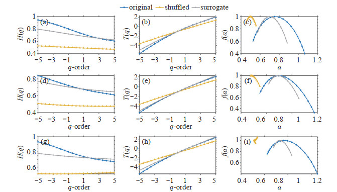
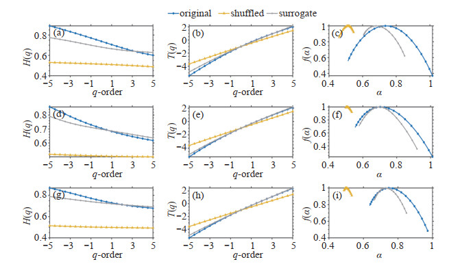
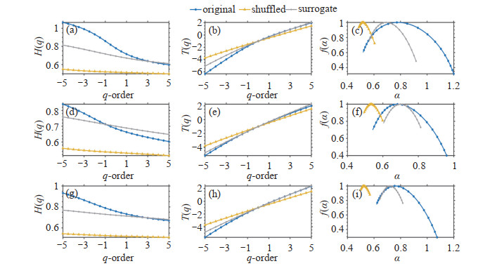
The multifractal characteristics result from the negative power-law distribution of temperature series and the correlation of fluctuations in different scales (He and Zhao^[31]; Varotsos and Efstathiou^[39]). The LRC of temperature time series indicates that the fluctuations of temperature records are not simply caused by external random disturbances. The cumulative effects of temperature formation and evolution mainly result in the fluctuations caused by inner nonlinear relations. Once there are certain differences in certain behaviors at a different period, there may exist multifractality given similarities between evolution behaviors. Studies have shown that the LRC as well as the negative power-law distribution can influence the multifractal properties of the temperature time series(Ray et al.^[40]). In this research, we have compared the parameters of shuffled and surrogate temperature time series to examine the contribution of the two factors in the formation and the strengthening of multifractal characteristics. The shuffled data can destroy the correlations; however, it preserves the fluctuation distribution. The surrogate data can keep the correlations; however, it will change the probability density function of the temperature records to a Gaussian distribution (Zhang et al.^[41]). On the one hand, if the multifractality of the temperature records only belongs to long-range correlation, the generalized Hurst exponent of the shuffled records will be a constant value, i. e., H(q) ≈0.5. On the other hand, if the multifractality of the temperature records only belongs to the negative power-law distribution, the generalized Hurst exponent of the surrogate records will be independent of q. However, if both kinds of multifractality are presented in the original temperature time series, the shuffled and surrogate series will show a weaker multifractality than the original one.

Figures 6-8 show that the exponent H(q)s of the shuffled series are not equal to 0.5 and are smaller than that of the original records. A very slight decrease in H (q) with an increase in q can be observed from the above figures, indicating a very weak multifractality. Therefore, the multifractality of the original time series is not only caused by long-range correlation but also caused by fat-tailed distribution.

Figure 6.  Diagram for the T_avg multifractal characteristics of the original, shuffled, and surrogate series. (a) - (c) respectively represents Guangdong, (d)-(f) Jiangsu, and (g)-(i) Liaoning.

Figure 7.  Diagram for the T_max multifractal characteristics of the original, shuffled, and surrogate series. (a) - (c) respectively represents Guangdong, (d)-(f) Jiangsu, and (g)-(i) Liaoning.

Figure 8.  Diagram for the T_min multifractal characteristics of the original, shuffled, and surrogate series.(a)-(c) respectively represents Guangdong, (d)-(f) Jiangsu, and (g)-(i) Liaoning.

Plots of τ(q)~q show that the multifractal strength decreases in order from the original series, the surrogate series, to the shuffled one. Similar results can be found for plots of f (α)~α. Taking into consideration the above findings, it is concluded that both LRC and fat-tailed distributions can cause the multifractal properties of temperature records, and the multifractality is more attributed to long-range correlations.

Table 2 presents the ΔH and Δα of the original and the transformed temperature time series. The strength of multifractal characteristic was quantitatively characterized by the scale of ΔH and Δα. From Table 2, it has been observed that the multifractal strength decreases in order from the original series, the surrogate series, to the shuffled one.

The climate system has various functioning mechanisms, thus causing multiple scaling behaviors and possessing multiple scaling exponents α(Yun et al.^[42]). In general, for 0 < α ≤ 0.5, the temperature series represents short-term memory, which means that the current events will not influence the long-term climate trend; while a value of a between 0.5 and 1.0 indicates long-term memory, which means that there is a similar trend for both past and future variability of the time series. The regional climate system has varying degrees of stability within a certain period of time, showing the characteristics of long memory (Atika et al.^[43]; McColl et al.^[44]; Beaulieu et al.^[45]). Therefore, the long-range correlation of the temperature series is likely to be caused by the long memory; that is to say, the temperature is regulated in a correlated and persistent way (Rypdal et al.^[46]; Gil-Alana^[47]).

In all the cases, the temperature series exhibit strong multifractality. The LRC in Liaoning is the highest, followed by that in Guangdong and Jiangsu, which indicates that the most stable temperature series is that of Liaoning, followed by the time series of Guangdong and Jiangsu. It is likely that Liaoning is located in the temperate continental monsoon zone in which the climate system is least influenced by the marine factors and thereby is very stable. On the contrary, the climate system of Guangdong is influenced by marine factors, and its stability is significantly influenced by Sea Surface Temperature (SST) anomalies. Jiangsu is located in a transitional zone between the temperate zone and the subtropical zone. It is also near the 0 ℃ January isotherm in China and is alternately controlled by cold and warm air masses, forming a complicated and unstable climate system.

The multifractal singularity spectrum reflects both the local and the global singularity of time series (Ampilova et al.^[48]). The singularity represents the extreme values of a function within a given range. And the multifractal singularity spectrum gives all the estimation of singularities of a climatic time series. The exponent α(q) reflects the local singularity of meteorological time series (Δα is the multifractal spectrum width and α_max and α_min represent the maximum and minimum α values, respectively). A higher Δα indicates a more uneven data distribution and a greater fluctuation. If the change of climate system is not consistent with he influence of natural law, then the fractal spectrum width tends to become narrower when the fluctuation range of climate series becomes smaller. The fractal spectrum with a certain width can reflect an asymmetric fractal structure. The more different the singularity strength, the more asymmetric the fractal structure (Shao and Ditlevsen^[49]).

The T_avg, T_max and T_min of Guangdong had the strongest multifractal strength, which indicated that its temperature fluctuation was the largest. The variation atmospheric circulation and sea temperature are the important factors that influence air temperature (Yun et al.^[42]; Chen et al.^[50]). Changes in the South China Sea, SST of the Western Pacific Ocean and subtropical high pressure belt will either slow down or continue to produce high temperature weather (Chen et al.^[51]; Xue and Fan^[52]). Guangdong is located in the low latitude area, which absorbs more solar radiation than other areas do and has active regional atmospheric circulation. Regional convective activity increases sharply when the sea surface temperatures of the South China Sea and the West Pacific are higher than usual, which is beneficial for the development of cyclones in the region. The warming will make this regional atmospheric circulation more unstable and change the water vapor transport and radiation balance. Under the above circumstances, the temperature will change more dramatically. The multifractality strength of the T_max series in Jiangsu was higher than that in Liaoning. However, the multifractality strength of the T_avg and T_min series in Jiangsu was lower than that in Liaoning, which indicated that the fluctuations of the T_max series in Jiangsu were larger than that in Liaoning and in the meantime the fluctuations of the T_avg and T_min series in Jiangsu were smaller than that in Liaoning. Jiangsu is greatly impacted by the Pacific tropical marine air mass. However, it is also slightly impacted by cold polar air masses. Influenced by the Arctic Oscillation and the North Atlantic Oscillation, Liaoning has a temperate continental monsoon climate characterized by hot and rainy summers, cold and dry winters. In winter, the polar continental air masses dominate the region, while in summer, the polar marine air masses or the tropical marine air masses dominate Liaoning with prevailing east and southeast winds (Xu et al.^[53]). The Yellow Sea Warm Current has an impact on the T_avg and T_min of Jiangsu, which simplifies the structure of the temperature series (Xie et al.^[54]).

In addition to the effect of atmospheric circulation, topography, urbanization and other factors can also cause the non-periodic changes of temperature. The topographic factors affect the detailed characteristics of the spatial distribution of air temperature in a small scale (Córdova et al.^[55]); the properties of underlying surface also affect the air temperature and its distribution (Chang and Lu^[56]). Besides, the topographic factors may also influence the multifractal strength of temperature series. As the average elevation of the northern Nanling Mountains in Guangdong is more than 1, 000 meters, it can prevent the cold wave from moving southward to a certain extent, which makes the average annual temperature in the south of Nanling Mountains higher than that in its north. Jiangsu is mostly a flat region, dominated by the Jiang-Huai Plain, and therefore cold air can enter directly. The topography of Liaoning essentially consists of the central lowland, flanked by mountain masses to the east and west with an uneven distribution of the surface temperature. The horseshoeshaped mountains and hills are inclined to the Bohai Sea, and the thermal properties of the grounds vary greatly in different regions of the province. The annual mean temperature of the area decreases gradually from southwest to northeast; the multi-year average distribution law of maximum temperature basically shows a trend that the plain is higher than the mountainous area and the coastal area is lower than the inland. The distribution law of minimum temperature shows that the minimum temperature decreases with the increase of latitude, and the minimum temperature in plain is higher than that in mountain area (Ni and Zhang^[57]; He et al.^[58]; Changchao et al.^[59]).

The acceleration of urbanization in Guangdong, Jiangsu and Liaoning has led to changes in the nature of the underlying surface in these urban areas, which result in the temperature rising through the change of energy balance. In addition, the change of thermal structures and underlying surface compositions can also lead to the urban heat island effect. Sun et al. and Liu and Murayama concluded that urbanization has a significant impact on the ground surface temperature records (Sun et al.^[60]; Liu and Murayama^[61]). Related researches in Japan and South Korea have also confirmed the impact of urbanization on temperature change (Chung et al.^[62]; Oishi^[63]; Matsumoto et al.^[64]). The effects of urban warming during the extreme heat wave events in the Yangtze River Delta (YRD) of China from July to August 2013 were assessed (Wang et al.^[65]). There was a positive feedback between urban warming and the intensity of heat wave, making the intensity of urban heat wave greater than that of rural areas, and the intensity of urban warming during the extreme heat wave events was greater than that of the climate mean value. The case studies (Luo and Lau^[66]; Zhong et al.^[67]; Yang et al.^[68]) in China showed that the intensification of urban heat island effect has a direct impact on local average temperature.

In conclusion, atmospheric circulation is the most important factor that affects the temperature change in the three regions. At the same time, the topographic differences of these three regions have different impact on their temperature changes. The topography of Guangdong and Jiangsu is relatively flat with relatively few terrain factors, and therefore they have little influence on the temperature change; the terrain factors of Liaoning are complex, which have a great influence on the temperature change. The urbanization levels of Guangdong and Jiangsu are relatively high, and the urbanization of these two regions has a significant influence on the local temperature change, while the urbanization level of Liaoning is relatively low, and its urbanization has a relatively light impact on its local temperature change.

In this research, the author has studied the variation law of the multifractal strength and LRC of the T_avg, T_max and T_min daily data in the typical temperature zones along the east coast of China, and has focused on the influence mechanism of atmospheric circulation, sea surface temperature (SST), and other factors on the multifractal characteristics of temperature in different regions. However, it is not just atmospheric circulation and SST that influence the variation of multifractal characteristics, but also human activities (such as the urbanization processes) and, more macroscopically, topography, and other factors. Therefore, in the future, the influence of human activities, topography and other factors on the multifractal characteristics of temperature will be taken as the research focus.

In this research, the MF-DFA method was adopted to identify the internal stability of temperature series and the strength of its self-regulation mechanism in the typical areas of different latitudes along the eastern coast of China, study how the long-range correlation in the series evolves, and discuss the influence of various natural elements. This study selected the daily average temperature, maximum temperature, and minimum temperature of Guangdong, Jiangsu and Liaoning, typical regions spanning subtropical zone, warm temperate zone and temperate zone, as its research objects, and adopted the generalized Hurst exponent, mass exponent, singularity exponent and multifractal spectrum system to study the multifractal strength and long-range correlation of T_avg, T_max and T_min in the above three regions. The main conclusions were as follows:

(1) The daily temperature time series showed strong multifractal properties. The temperature series in Liaoning exhibited the strongest multifractality, so the LRC in Liaoning was the highest, followed by that in Guangdong, and Jiangsu. The most stable temperature series was that of Liaoning, followed by the time series of Guangdong and Jiangsu. This may be related to the location of the research areas where they are affected by the marine factors and the cold and warm air masses to different degrees.

(2) Guangdong showed the highest degree of multifractal strength, so Guangdong's temperature experienced the largest fluctuations among the three provinces. The multifractality strength of the T_max series in Jiangsu was higher than that in Liaoning, while the multifractality strength of the T_avg and T_min series in Jiangsu was lower than that in Liaoning. Jiangsu had the larger fluctuations in T_max series than Liaoning did, while it had smaller fluctuations in T_avg and T_min series than Liaoning did. In addition to the differences in atmospheric circulation and sea surface temperature change in these three regions, this phenomenon was also affected by topographic factors: Jiangsu is mainly plain with a flat topography; however, Liaoning has many mountains and hills of which topography fluctuates greatly, and the thermal properties of the underlying ground surface vary greatly in different regions of the province.

(3) Guangdong and Liaoning both had the strongest T_min multifractal strength, followed by T_avg and T_max. However, in Jiangsu, it had the strongest T_max multifractal strength, followed by the T_avg and T_min. This may be related to the comprehensive effects of natural factors, urbanization and other factors.

(4) This dissertation researched the dominant factors of the T_avg, T_max and T_min multifractals, and through random re-ordering and phase randomization for the original temperature series, it calculated the generalized Hurst exponent H(q), singularity exponent α, and singularity spectrum f(α) to examine the multifractal sources of the temperature time series in comparison with the original, shuffled, and surrogate time series. Finally, the author found the multifractality of temperature time series was caused not only by negative power-law distribution but also by long-range correlation in which the contribution of the long-range correlation of the series itself to the formation of the multifractal characteristics of daily temperature series was greater than that of the negative power-law distribution.

In this study, the typical temperature zones of the eastern coastal regions of China were selected as its research areas, covering tropical, subtropical and temperate zones. And the MF-DFA method was adopted to study the multifractal characteristics and long-range correlations of daily temperature series and to identify the stability of climate systems in these different regions, which can help deepen the understanding of the temperature change patterns and their causes in different temperature zones in China under the background of climate change. The research on these aspects is not only a hot-spot issue in the field of climate change, but also an important content of disaster risk quantitative assessment, so the research will be an important reference for environmental protection and sustainable development.