Ingredients-based Methodology and Fuzzy Logic Combined Short-Duration Heavy Rainfall Short-Range Forecasting: An Improved Scheme

The predictability of the Earth's atmosphere has been a hotspot-forefront topic in atmospheric sciences (Lorenz ^[1,2]; Palmer and Hagedorn ^[3]; Delsole and Tippett ^[4]). Advances in numerical weather prediction (NWP) models have greatly improved our ability to forecast basic elements such as temperature and high-level pressure (Bauer et al. ^[5]). However, accurate forecasting of convective weather remains a big challenge. This difficulty arises from the interaction of many elements under different synoptic patterns and multi-scale features (Doswell ^[6]).

Short-duration heavy rainfall (SHR) is defined by the China Meteorological Administration (CMA) as rainfall that amounts to no less than 20.0 mm within one hour (Zheng et al.^[7]; Sun et al. ^[8]). SHR, as the main component of torrential rainfall and severe torrential rainfall events (Zhou et al. ^[9]), is the most common and the most damaging convective weather phenomenon in China (Liao et al. ^[10]; Wu et al. ^[11]). Many severe torrential rainfall events caused by severe SHR have been reported, with some setting new records. For example, a sudden short-duration heavy rainfall with an intensity of up to 151.0 mm h^–1 caused a mall in Jinan, Shandong Province, to be flooded, resulting in the drowning of more than 30 people (Liao et al. ^[10]). Five years later, on July 21, 2012, Beijing experienced an extreme rainfall event with a death toll of 79, where the maximum hourly rainfall reached approximately 103.0 mm (Chen et al. ^[12]). In Guangzhou, the record for maximum hourly rainfall was set at 184.4 mm on May 7, 2017 (Tian et al. ^[13]). However, this record was quickly surpassed on July 20, 2021, when an unprecedented extreme hourly rainfall of 201.9 mm was reported (Fu et al. ^[14]; Yin et al. ^[15]).

SHR short-range forecasting is operationally produced and issued at the National Meteorological Center (NMC) of CMA to alert people to the risk of potential flash floods, and to provide additional reference to enhance the accuracy of quantitative precipitation forecast (QPF). These SHR forecasts are issued three times a day during warm seasons, specifically at 06:00, 10:00, and 18:00 Beijing time (BJT, BJT=UTC+8). Environmental conditions, including moisture content, potential lifting mechanisms, and instability conditions, are comprehensively analyzed, and SHR forecasts are manually produced based on this comprehensive assessment. However, the skills in forecasting SHR still need to be improved for many reasons, among which the measurement of the relative importance of environmental moisture, lifting mechanisms, and instability is more challenging compared with the understanding of the influence of topography and atmospheric circulation (Chen et al. ^[16]) and the interaction of large-scale and mesoscale systems (Doswell ^[6]).

There are methods of objective forecasting developed to provide reference for convective weather forecasts. These methods include overlapping methods (Li et al. ^[17]), logistic regression models (Schmeit et al. ^[18]; Pang et al. ^[19]), random forests (Hill et al. ^[20]), fuzzy logic approach (Haupt et al. ^[21]), and deep learning models. The overlapping method is not robust as the physical meanings of parameters are not considered. Logistic regression models also face similar problems. Tian et al. ^[22] found that parameters indicating the lifting condition can be significantly underestimated if all parameters are generally compared together. Random forests as a kind of artificial intelligence method are more energetic as they have the possibility of measuring the relative importance of environmental conditions. Fuzzy logic approaches among these methods are applied more broadly attributed to their good performance in efficiently using information, simplicity to design and implement, and straightforwardness to interpret and modify (Haupt et al. ^[21]). Lin et al. ^[23] and Kuk et al. ^[24] documented the skillfulness of fuzzy logic methods in providing short-range thunderstorm prediction by using environmental parameters. Tian et al. ^[25] proposed a SHR short-range forecasting method by combining the ingredients-based methodology and fuzzy logic approach (hereafter IM-FLA).

The IM-FLA method has been documented as skillful but too subjective to be promoted for wide application. For the IM-FLA method, parameters are firstly divided into groups indicating the environmental moisture content, instability, and dynamic lifting conditions. Predictors are then determined by comparing the discrimination of SHR from both no rainfall (intensity less than 0.1 mm h^–1) and ordinary rainfall (intensities between 0.1 and 19.9 mm h^–1) among the grouped parameters. Then the membership functions of predictors are arbitrarily determined with specific percentiles as thresholds. Some aspects could be improved to make the IM-FLA method more objective and robust. The first is that the no rain samples could be excluded during the selection of the predictor. Great advances have been made for NWP models in providing rain or no rain forecasts (Wang et al. ^[26]; Liu et al. ^[27]; Wang and Yan ^[28]). Thus, we can just focus on two kinds of rainfall: ordinary rainfall and SHR. The second is that newly available studies show that vertical wind shear should be excluded from the list of studied parameters. Púčik et al. ^[29] summarized the influence of vertical wind shear on different convective phenomena and pointed out that the occurrence of convective hazards such as large hail, severe wind gusts, and tornadoes increases with increasing vertical wind shear. However, this trend is not applicable to excessive rainfall (Doswell et al. ^[30]). The third is that the arbitrarily obtained membership functions with the piecewise linearization method are unreasonable. The maximum membership functions with the IM-FLA method can reach up to 1.0. However, the fact is that no single parameter can be used to distinguish SHR from ordinary rainfall completely. Approaches with some statistical basis should be investigated. The last is the determination of weights. Objectively determined weights will make the forecasting method more objective and more robust though the weights are not as important as predictors. A new IM-FLA method (hereinafter new IM-FLA) considering the above-mentioned aspects will be introduced in this paper.

This paper is organized as follows. Section 2 introduces the datasets and verification methods used in this study. A detailed description of the new IM-FLA is given in Section 3. The evaluation of its performance is given in Section 4 and Section 5. Section 6 is the summary and discussion.

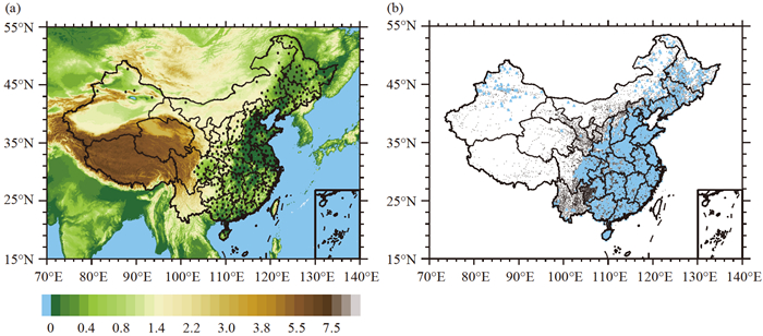
The data used in this study included two parts. One was the collected hourly rainfall observations reported by 411 national meteorological stations (Fig. 1a) with altitudes less than 2000 m and the National Centers for Environmental Prediction (NCEP) final analysis (FNL) data, which were used for the development of the new IM-FLA forecasting method. The other was the NWP data provided by the NCEP global forecast system (GFS) and hourly rainfall observations reported by both the national meteorological stations with altitudes less than 2000 m and automatic weather stations (Fig. 1b). The data were used for the reproduction of SHR forecasts and performance evaluation.

Figure 1.  Distribution of (a) 411 observational stations (black dots) and (b) 1887 verification stations (blue dots) and automatic meteorological stations (black dots).

The period of coverage of NCEP FNL data and national meteorological stations used for the development of the new IM-FLA method was between May 1 and September 30 in the years 2002 and 2009. Candidate parameters included total precipitable water (TPW), specific humidity (Q), the best lifted index (BLI), the best convective available potential energy (BCAPE), low-level divergence, and so on (Table 1). Vertical wind shear indicators were excluded. The classification was based on the representative meaning of parameters. Some parameters such as BLI and BCAPE were classified as instability indicators. Others such as TPW, Q, and relative humidity were classified as moisture indicators. The 850 hPa and 925 hPa divergence were studied as indicators of dynamic lifting.

Spatial and temporal matching processes were executed to reconcile the disparities in resolutions between available NCEP FNL data and the sparsely distributed observational data. The NCEP FNL data had a spatial resolution of 1.0°×1.0° and a temporal resolution of six hours (02:00, 08:00, 14:00, and 20:00 BJT). The temporal resolution of rainfall observations was one hour, yielding a total of 24 hourly records per day. These records were firstly divided into four periods with the time of NCEP FNL as the centers. The presence or absence of SHR was ascertained by examining the rainfall figures from the six hourly records within each period. A sample was classified as "no rain" only if all six records indicated an absence of rainfall. Conversely, a sample was deemed an "SHR" instance if any of the records indicated SHR. Otherwise, an ordinary rainfall sample was obtained. This process resulted in a sample size of 350,000 instances for ordinary rainfall and 11, 400 for SHR. The corresponding values of parameters at 411 stations were obtained using a bilinear interpolation method.

The data from the NCEP GFS, initialized at 08:00 BJT between April 1 and September 30, 2015, was used to reproduce the SHR forecasts. The new IM-FLA method used for the reproduction of SHR forecasts will be described in Section 3. The NCEP GFS data had a spatial resolution of 1.0° by 1.0° and a temporal resolution of 3 hours. With these data, the necessary parameters and indices were obtained and 3-hour interval SHR forecasts were calculated. However, the 3-hour interval SHR forecasts within 96 hours were integrated into eight 12-hour interval SHR forecasts by leaving the maximum potential grid by grid, facilitating the comparison with the 12-hour interval operational SHR forecast. Ultimately, the 12-hour interval SHR potential forecasts within 96 hours with a spatial resolution of 1.0°×1.0° were obtained.

SHR predominantly occurs in middle and lower latitude regions and has remarkable regional characteristics (Chen et al. ^[31]). A spatial verification method was adopted and the 1887 verification stations situated at altitudes less than 2000 m (Fig. 1b, blue dots) and more than 40,000 automatic weather stations (Fig. 1b, black dots) over eastern China were both used during the verification. All the available observations within 40 km of each verification station were scanned for spatial verification. The SHR potential at all verification stations was obtained by using the bilinear interpolation method. The determined and probabilistic features were then evaluated.

The deterministic performance of SHR forecasts was evaluated with thresholds at 2.5% increments to create a contingency table. The hits (A), false alarms (B), misses (C), and correct rejections (D) were then counted according to Table 2. Threat score (TS), bias (Bias), probability of detection (POD), and false alarm ratio (FAR) were then calculated as follows:

The Brier Skill Score (BSS) and reliability diagrams, which are standard tools for verifying probabilistic forecasts, were adopted in this study to investigate the probabilistic properties. The BSS evaluates the quality of the forecasts and thus the reliability of probability forecasts. It quantifies the improvement of a forecast's Brier Score (BS) over that of a reference climatological forecast (BSc). The BSS is calculated using the formula:

The BSS will be 1.0 for a perfect forecast. A BSS of zero means that there is no improvement compared with climatological probability, while a negative BSS indicates a poorer quality than the climatological probability. The reliability diagram categorized the forecasts into bins according to the probability. The frequencies with which the event was observed to occur for sub-groups of forecasts were then plotted against the vertical axis. The reliability of the forecast probability and the frequency of occurrence should be equal for perfect reliability, and the plotted points would lie on the diagonal.

The fuzzy logic approach was adopted as a tool for mapping the potential of SHR as shown in Eq. 6, where P is the probability of SHR while M_i and W_i are the membership functions of selected predictors and corresponding weights, respectively. n is the number of selected predictors.

The probability P can be obtained only if the membership functions and weights of predictors were determined.

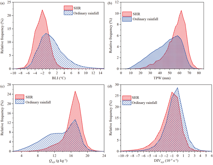
The parameters indicating environmental conditions were firstly divided into three groups according to their physical properties (Table 1). The predictors were then selected by comparing the size of overlapped areas (S) of the relative frequency of a parameter for ordinary rainfall and SHR (Fig. 2). A smaller S always indicates better discrimination. The parameter with the smallest S within its group is unquestionably the best candidate predictor.

Figure 2.  The distribution of relative frequency (probability density) of (a) BLI, (b) TPW, (c) Q₉₂₅, and (d) DIV₉₂₅. The meshed sections indicate the overlapped areas.

The comparative analysis of overlap sizes reveals that certain parameters exhibited superior discriminatory power over others (Table 1). The BLI had a minimum S of 0.52 among the instability indicators. The second and the third were θ_se925 and θ_se850 with corresponding S of 0.63 and 0.64, respectively. The widely used BCAPE was only listed as the fourth with the S of 0.67. The KI had an S of 0.70. The S for TT was high up to 0.96, indicating minimal discrimination efficacy. BLI was thus selected as the candidate predictor for instability conditions. TPW and Q₉₂₅ had the same and smallest S of 0.70 among all the moisture content indicators, leading to their selection as candidate predictors. All the other parameters indicating atmospheric saturation, specific humidity, and water vapor flux divergence had an S equal to or greater than 0.75, thus not meeting the selection criteria. For dynamic lifting indicators, the smallest S was 0.83 found at DIV₉₂₅, which was consequently selected as a candidate predictor for environmental dynamic lifting conditions. In total, four parameters, i.e., BLI, TPW, Q₉₂₅, and DIV_925, were selected as candidate predictors.

The characteristics of the relative frequency of the four candidate predictors for ordinary rainfall and SHR were different (Fig. 2). The smaller the BLI, the higher the relative frequency for SHR compared with that for ordinary rainfall. The peak of relative frequency of BLI for SHR was about 22% with the BLI around –2.0℃ (Fig. 2a). There was a part of the SHR that occurred with a positive BLI. Comparatively, the maximum relative frequency of BLI for ordinary rainfall was only about 13% with the BLI around 0℃. The similarity of the distribution of BLI, TPW, and Q₉₂₅ was that the maximum relative frequencies for SHR were much higher than that for ordinary rainfall. The relative frequency for ordinary rainfall was overtaken by that for SHR at a TPW of 50 mm. The peak of relative frequency for SHR was about 10% with the TPW around 62 mm while that for ordinary rainfall was about 6.0% with the TPW around 58 mm (Fig. 2b). The peak relative frequency of SHR and ordinary rainfall for Q₉₂₅ were both at 17.0 g kg^–1 with values of about 25.3% and 13.4%, respectively. However, the distributions of SHR and ordinary rainfall for DIV₉₂₅ appeared largely parallel, with only minor variations (Fig. 2c).

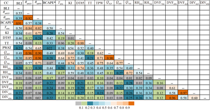
The correlation coefficients (CCs) of the studied parameters were also studied to help with the selection of predictors. Only one could be selected as the predictor for the two parameters with high CC. The CC was obtained with Eq. 7 as follows:

The results show the CCs for most of the studied parameters were less than 0.50 (Fig. 3). However, there were still some parameters that had close relationships. For example, the CCs between divergence and water vapor flux divergence of 925 hPa and 850 hPa were 0.97 and 0.96, respectively. The close relationship between them could be explained by the fact that flow divergence itself was a very important part of water vapor flux divergence (Ma et al. ^[32]). The CC of θ_se between 925 and 850 hPa was high up to 0.92. The CC for 925 and 850 hPa θ_se and Q was also high. Moreover, the CC for BLI and BCAPE was 0.91. Fortunately, only BLI was selected as the candidate predictor indicating instability conditions.

Figure 3.  CCs for different parameters. The CCs for parameters with BCAPE are obtained by using polynomial curve fittings (marked with an asterisk (*) for clarity).

CCs between the candidate predictors indicate they were proper predictors (Fig. 3). The maximum CC for the four selected candidate predictors was 0.62 between PWAT and Q_925. The medium to strong relationship between TPW and Q₉₂₅ could be attributed to that the moisture was mainly concentrated near the Earth's surface (Zhai and Eskridge ^[33]), and TPW was the integration of specific humidity from the surface to about 200 hPa. However, both the total moisture content indicated by TPW and the low-level moisture content was important for convective storms, the direct producer of SHR. A certain amount of moisture content was the prerequisite for heavy rainfall. An amount of at least 28 mm TPW was necessary for SHR (Tian et al. ^[34]). The behavior of MCSs was highly sensitive to low-level moisture (Schumacher and Peters ^[35]). Both TPW and Q₉₂₅ were selected as predictors. The second highest CC was 0.48 between BLI and Q₉₂₅. It was a medium to weak correlation. The low-level moisture content played an important role in the calculation of BLI (Galway ^[36]). Fortunately, BLI and Q₉₂₅ represented instability and moisture conditions, respectively. The CCs for other candidate predictors were all smaller than 0.40. The four candidate predictors were finally selected as predictors.

Membership functions are important in connecting specific values of predictors to the predicted SHR probability. There are several ways to obtain membership functions. Rossi et al. ^[37] used empirical cumulative distributions of parameters to produce triangular-shaped membership functions for classifying the severity of convective storms. There are no empirical cumulative distributions of parameters available for SHR. Obtaining membership functions with conditional probability is an instructive test. Lin et al. ^[23] used conditional probability to predict afternoon thunderstorms. However, the total probability of SHR was about 3.15% as the sample size of ordinary and SHR were 350,000 and 11,400, respectively. The detailed conditional probability was too small to be used directly as the membership functions (see the Appendix for more detail). Thus, Tian et al. ^[25] used the percentiles arbitrarily to obtain the membership functions. Here we followed Kuk et al. ^[24] and used relative frequency to produce membership functions.

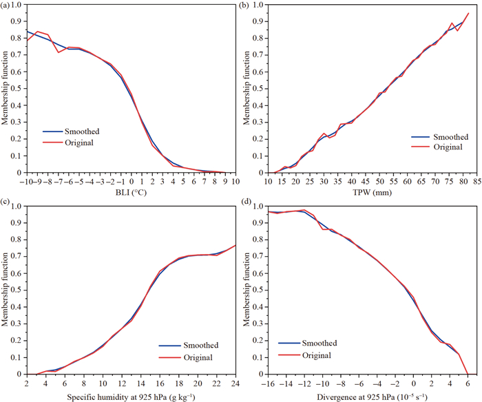
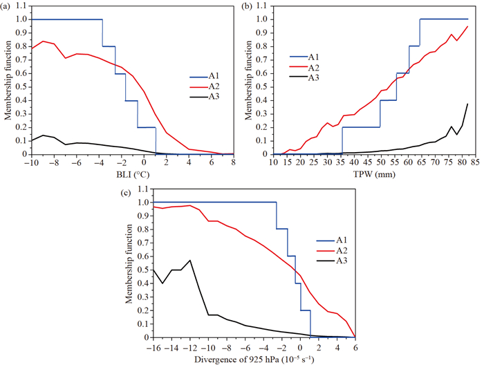
The membership functions were obtained based on relative frequencies. It was the portion of the relative frequency of SHR to the sum of the relative frequencies of SHR and ordinary rainfall. The variations of membership functions of the four predictors obtained with this process were generally monotonic though many saw teeth in detail (Fig. 4). The maximum membership for BLI was about 0.84 with the BLI at –9.0℃. The membership generally decreased as the BLI increased. There was some membership even if the BLI was greater than 3℃ (Fig. 4a). Both the TPW and Q₉₂₅ were predictors indicating the moisture conditions but had many different characteristics on membership functions. The membership function for TPW increased monotonically as the value increased from about 15 mm to about 85 mm (Fig. 4b). The maximum membership was about 0.95. The membership for Q₉₂₅ also increased monotonically as the value increased (Fig. 4c). The membership increased quickly as Q₉₂₅ was smaller than 18 g kg^–1, and then very slowly. The maximum membership for Q₉₂₅ was about 0.77 obtained around 24 g kg^–1. The maximum membership for DIV₉₂₅ was high up to 0.97 (Fig. 4d), a value higher than the predictors indicating environmental instability and moisture content conditions. The membership function seemed to be a constant when DIV₉₂₅ was less than –12.0×10^–5 s^–1, but then it dropped quickly to 0.0 with the DIV₉₂₅ at about 6.0×10^–5 s^–1. The maximum memberships of TPW and DIV₉₂₅ were close to 1.0, but still less than 1.0 indicating none of the predictors had a complete discrimination on SHR and ordinary rainfall. During the operational SHR forecasts, the area with positive BLI or DIV₉₂₅ was usually considered with low possibility of SHR. Fig. 4 shows that the membership was 0.45 when the BLI was 0℃, and membership was smaller than 0.1 when the BLI was greater than 3℃. The membership was 0.44 when the DIV₉₂₅ was 0.0×10^–5 s^–1, and it then rapidly reduced to 2.0 at the DIV₉₂₅ of 3.0×10^–5 s^–1. The five-point average smoothed membership functions were finally used for obtaining SHR probability to reduce the influence of sawteeth (Fig. 4). Furthermore, the thresholds listed in Table 3 should be met if SHR was expected to reduce false alarms. The thresholds were obtained from preliminary studies (Tian et al. ^[25]; Tian et al. ^[34]).

Figure 4.  Original (red lines) and smoothed (blue lines) membership functions of (a) BLI, (b) TPW, (c) Q₉₂₅, and (d) DIV₉₂₅.

Objectively determined weights of predictors will make the IM-FLA method more robust. In this study, the weights were obtained by calculating the size of overlapped areas of predictors (Table 1). Smaller overlapped size always indicates better discrimination of the parameter and should have a higher weight. The weights were determined as follows. Firstly, the overlapped area of a predictor, S, as listed in Table 1, was calculated. Secondly, the subtraction of 1.0–S was calculated. Thirdly, the weights of predictors with the 1.0–S as the portion were obtained. The corresponding weights of the four predictors were 0.38, 0.24, 0.24, and 0.14 as listed in Table 4.

The weights of the three ingredients were much different. BLI was the only predictor that indicated environmental instability conditions. The total weight of instability was 0.38. Both TPW and Q₉₂₅ were environmental moisture content indicators. The total weight of moisture content was 0.48. The weight of dynamic lifting was 0.14. The moisture content had the highest weight while dynamic lifting had the smallest weight. The reason could be that moisture content was an absolutely important factor of SHR. No SHR could be expected without enough moisture in the atmosphere. It was under environments with a certain amount of moisture that the instability and dynamic lifting became pertinent for SHR. Though the influence of specific values of predictors on results was more significant than the weights, a control group with equal weights was set as for comparison to verify the validity of the findings.

The two cases used by Tian et al. ^[25] were adopted in this study to facilitate the comparison with the IM-FLA method. The two cases were the deep summer typhoon Soudelor on August 8, 2015, and a challenging southern China spring case on May 15, 2015. Only brief information is given in this section as a detailed introduction to these two cases can be found in Tian et al. ^[25].

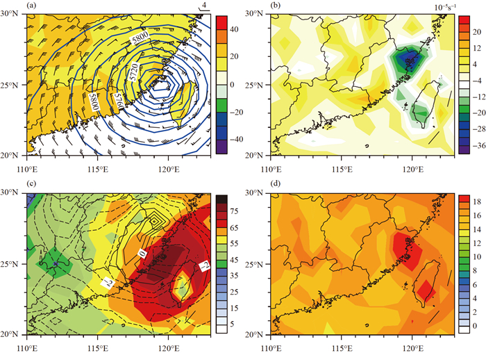
The predicted synoptic pattern valid at 20:00 BJT on August 8, 2015 shows it was a very strong typhoon. The predicted 24-hour 500 hPa center pressure was less than 566 hPa (Fig. 5a). The 850 hPa wind was very strong with a maximum wind speed greater than 44 m s^–1 (Fig. 5a), indicating a strong typhoon. At this time, the north of Soudelor had the strongest lifting conditions as the DIV₉₂₅ was even less than –20.0×10^–5 s^–1 (Fig. 5b) with the high Q₉₂₅ center also located in this area (Fig. 5d). There were two high Q₉₂₅ centers with one just located at the strong lifting area. The maximum Q₉₂₅ was higher than 18.0 g kg^–1 (Fig. 4d). However, the high TPW area just lied along the coastlines with amaximum value greater than 75 mm (Fig. 4c). Meanwhile, the instability indicated by BLI was not strong as only a minimum of –2℃ around the focused center areas of Soudelor was given (Fig. 5c).

Figure 5.  The NCEP GFS predicted 24-hour synoptic pattern and parameter distribution valid at 20:00 BJT on August 8, 2015. (a) 850 hPa wind field (where a full bar represents 4 m s⁻¹, and a flag represents 20 m s⁻¹), 850 hPa temperature (℃, shaded), and 500 hPa isobars (solid black line). (b) 925 hPa divergence (10⁻⁵ s⁻¹). (c) BLI (℃) and TPW (shaded with legend at right) distribution. (d) 925 hPa specific humidity (g kg^–1).

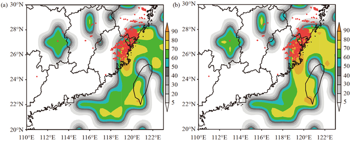
The 24-hour SHR probability distributions predicted by models, utilizing both unequal and equal weights, valid as of 20:00 BJT on August 8, 2015, show similar patterns but the difference in details (Fig. 6). The SHR probabilities over the oceans were also left to indicate the usefulness of the forecasts over areas where observations were not available. Southeast Zhejiang Province and northeast Fujian Province were the main area that should be the focus area for SHR. Most of the SHRs reported by automatic weather stations are located within the predicted areas. The predicted highest probability from models with both unequal and equal weights was higher than 90%. The main difference could be that the high probability area greater than 90% given by forecasts obtained from the model with unequal weights only covered northeast Fujian Province while that given by forecasts obtained from the model with equal weights covered both southeast Jiangsu Province and northeast Fujian Province.

Figure 6.  Comparison of predicted 24-hour probability valid at 20:00 BJT on August 8, 2015 from models with (a) unequal and (b) equal weights.

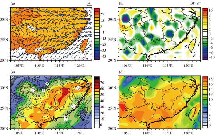
This case displays the difficulty of SHR forecasting during spring seasons. The predicted 48-hour synoptic pattern shows the 588 hPa line usually used to indicate the location and strength of subtropical high extended from the southeast of Fujian Province to the southeast of Guangxi Zhuang Autonomous Region (Fig. 7a). There was a convergence line on the 850 hPa wind field that just lied behind the 584 hPa line of 500 hPa, indicating an attention earned background for convection. The 925 hPa divergence shows a large area with a negative divergence, indicating widespread favorable but not strong low-level lifting conditions compared with that in the Soudelor case (Fig. 5b). The minimum DIV₉₂₅ at this area was only about –6.0×10^–5 s^–1 (Fig. 7b). The BLI for a large area along the 850 hPa wind convergence line was between –2℃ and –3℃ (Fig. 7c) while the BLI over Guangxi and Guangdong were much stronger as the values were less than –5℃. Most of the area had the TPW less than 60.0 mm (Fig. 7c). The Q₉₂₅ at a large area was less than 16.0 g kg^–1 (Fig. 7d). None of the predictors can reach up to the maximum values of memberships according to Fig. 4. This illustrates why the spring SHRs are so difficult to forecast: despite the presence of seemingly favorable environmental conditions, accurately assessing the likelihood of such events remains a challenge.

Figure 7.  NCEP GFS predicted 48-hour synoptic pattern and parameter distribution valid at 20:00 BJT on May 15, 2015. (a) The 850 hPa wind field (a full bar represents 4 m s⁻¹, and a flag represents 20 m s⁻¹), 850 hPa temperature (℃, shaded), and the 500 hPa isobars (solid black line). (b) 925 hPa divergence (10⁻⁵ s⁻¹). (c) TPW (shaded with legend at right) and BLI (℃). (d) 925 hPa specific humidity (g kg^–1).

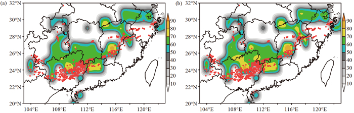
The possibility of SHR was correctly delivered by objective SHR forecasts from models with unequal and equal weights. The maximum probability was higher than 90% in the south of Jiangxi Province and the north of Guangxi Zhuang Autonomous Region. Most of the areas had a probability of less than 70% (Fig. 8). The higher probability area from the model with equal weights was larger than that obtained from the model with unequal weights. However, both the high probability areas given by the models with different weights were much smaller than those given by Tian et al. ^[25]. The reason could be caused by the determination of membership functions. The memberships were smaller than that subjectively obtained ^[25]. Statistical evaluation could tell which membership function-obtaining method could be better.

Figure 8.  Comparison of predicted 48-hour probability (%) valid at 20:00 BJT on May 15, 2015 for the forecasts obtained from models with (a) unequal and (b) equal weights.

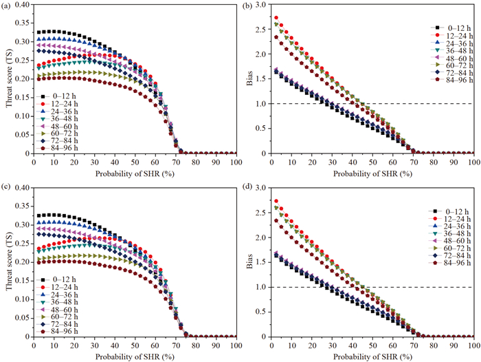
Statistical evaluations were carried out to display the advantages of the new scheme. The deterministic results show the new IM-FLA was skillful and a little better than that given by the IM-FLA method. The 12-hour interval SHR forecasts obtained from the models with unequal and equal weights groups using NCEP GFS data initiated at 08:00 BJT were evaluated. The coverage of 0–12, 24–36, 48–60, and 72–84 h were daytime periods, while the coverage of 12–24, 36–48, 60–72, and 84–96 h were nighttime periods. The daytime and nighttime cluster remained. The results of TS and Bias for the group with unequal weights indicate that the daytime forecasts were better than the nighttime forecasts (Fig. 9). The TS with different coverage gathered into two groups exactly. The maximum TSs for the daytime periods were much higher than that for the nighttime periods (Fig. 9a). Meanwhile, the Biases also clustered into two groups corresponding to the TSs. The TS increased first and then decreased as the probability of SHR increased for most of the periods. The maximum TS for the 0–12 h period was about 3.28×10^–1, a little higher than 3.20×10^–1, the maximum TS that was given by the IM-FLA (comparison group in this study). The maximum TSs for other periods were all less than 3.20×10^–1. The TS reached 0 around the probability of about 72%. As a reference, the TS for the operational SHR forecasts was about 0.24. The maximum Biases given at the minimum probability point were between 1.50 and 3.00 for different coverage, and then they decreased to 0 around the probability of about 72%. The results for other forecast periods had similar characteristics, too.

Figure 9.  The variation of TS and Bias of different forecast periods for the groups with unequal and equal weights. (a) Variation of TS for the group with unequal weights, (b) variation of Bias for the group with unequal weights, (c) variation of TS for the group with equal weights, and (d) variation of Bias for the group with equal weights.

The performance of the group with equal weights was as good as the group with unequal weights (Fig. 9c and Fig. 9d). The characteristics of TS and Bias were much the same as those given by the group with unequal weights. The daytime and nighttime clusters for TSs and Biases were also clear. The maximumTS for the 0–12 hour was about 3.27×10^–2, very close to 3.28×10^–2, which was given by the group with unequal weights. The most remarkable difference could be that all the TSs and Biases reached 0 at about 75% while that for the group with unequal weights was around 72%. The results again demonstrate that the SHR forecasts are highly determined by environmental conditions rather than the weights of predictors.

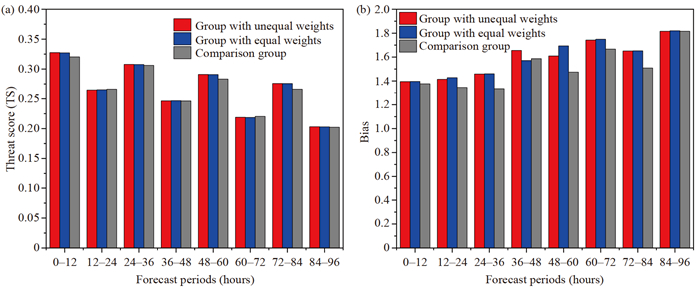
The variation of maximum TSs and the corresponding Biases shows the results obtained with the new IM-FLA were a little better than those given by the comparison group. The maximum TSs and corresponding Biases for different forecast periods for the group with unequal weights, group with equal weights, and that for the comparison group were picked out (Fig. 10). The maximum TSs given by the groups with unequal and equal weights were much the same. They were higher than that given by the comparison group for most of the forecast periods (Fig. 10a). The daytime and nighttime clusters were also clearly displayed in the variation of the maximum TSs. The daytime maximum TSs were higher than the neighbored nighttime maximum TSs for all the two groups with different weights and the comparison group. The reason could be that solar heating was the immediate cause of local thermal forcing (Li et al. ^[38]), and thus the afternoon peak of convection (Xu et al. ^[39]). Convection was the direct producers of SHR. The afternoon peak was clear as the diurnal variation of SHR shows (Ma et al. ^[31]). However, the characteristics could not be fully revealed by the NCEP reanalysis data as the daily cycle of precipitation shows (Dai et al. ^[40]; Zhou and Wang ^[41]). The variation was not significant for the BIASs. The Biases for different forecast periods were a little bigger than that given by the comparison group indicating larger false alarms (Fig. 10b). The Bias for the 0–12 h was about 1.40 and gradually increased to about 1.80 for the 84–96 h forecast. Despite the small difference, the verification results show the groups with unequal and equal weights were a little better than the comparison group as it was the best one among the results obtained with the IM-FLA method.

Figure 10.  Comparison of (a) maximum TS and (b) corresponding Bias for different forecast periods obtained with different settings.

The BSS gives a clearer picture of the advantages of the group with unequal weights. The maximum BSS for the group with unequal weights was 7.15×10^–2 for the 0–12 h forecasts (Table 5). Then the BSS gradually decreases, and the BSS for the 84–96 h forecasts was only about 1.45×10^–2. The results show that the longer the forecast period the worse the forecast skills. The BSS for the group with equal weights for the 0–12 h group was 7.12×10^–2, close to that for the group with unequal weights. However, the BSS given by the group with equal weights was worse than that given by the group with unequal weights for all forecast periods. It indicates a worse result for the group with equal weights. The comparison group that obtained with the IM-FLA had the same BSS of 7.12×10^–2 as that given by the group with equal weight. However, the BSS for the other forecast periods was all significantly smaller than that obtained with the groups with unequal and equal weights. The BSS of the comparison group for the 60–72 h and 84–96 h forecasts were negative, indicating poorer qualities than the climatological benchmarks. The group with unequal weights was the best, and and then was the group with equal weights; they were better than the comparison group.

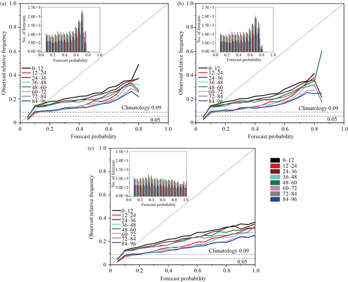
We also adopted the reliability diagram to investigate the detailed characteristics of the probability forecasts. The reliability diagrams show that the results were remarkably improved compared with the comparison group though the daytime and nighttime clusters were still clear. There were two aspects of improvements compared with the comparison group (Fig. 11). One was the significant improvement over forecasts as shown by the comparison group (Fig. 11c) was improved. The lines given by the groups with unequal and equal weights were closer to the diagonal. The other was that the distribution of sample size shows there was high confidence for the groups with unequal and equal weights. In contrast, the comparison group only had the intermediate confidence (Wilks ^[42]). It should be noted that the predicted SHR probability can range from 0 to 100% (Fig. 11c). In comparison, both the groups with unequal and equal weights given by the new IM-FLA only had the probability range between 0 and 90% (Figs. 11a and 11b).

Figure 11.  Distribution of reliability diagram for (a) group with unequal weights, (b) group with equal weights, and (c) comparison group. The bars at the upper left corner denote event probability distributions. The two dashed horizontal lines represent the SHR climatology during the daytime (upper) and nighttime (lower) period within the studied period.

An improved short-range SHR objective forecasting scheme combining the ingredients-based methodology and fuzzy logic approach was introduced in this study. Four aspects were improved to make the new IM-FLA method more robust and widely applicable. The first was that the no rainfall category was excluded. The second was that the environmental vertical wind shears indicating parameters were excluded. Fewer parameters were used. The third was that the membership functions of the predictors were statistically rather than arbitrarily obtained. The last was that the weights of the predictors were objectively determined. These processes improved the objectivity of the new IM-FLA and the performance of the forecasts. Benefiting from the four aspects, the new scheme can now be applied to the forecasting of many other convective phenomena for which only yes and no datasets are available.

The ingredients-based methodology provided the basis of predictor selection while statistics and fuzzy logic were used as the implementation tools. The parameters were divided into groups indicating the environmental moisture content, instability, and dynamic lifting conditions before predictors were selected. The following processes were then carried out. The predictors among each of the groups were determined by comparing the sizes of the overlapped areas of the relative frequencies for SHR and ordinary rainfall. The crucial part of the fuzzy logic approach bridging the physically meaningful predictors and the probability of SHR was the obtaining of the membership functions and the determination of weights. Key thresholds of parameters were also used to reduce false alarms. The verification for the 2015 warm season shows the new IM-FLA method was better.

This study again demonstrates that physical understanding and fuzzy logic approach combined method is a feasible and robust way of solving the challenging short-duration convective weather phenomena short-range forecasting problem. The maximum values of memberships of all the predictors were smaller than 1.0, indicating the impossibility of a hundred percent probability of SHR. This could be determined by the nature that large-scale systems form favorable environmental conditions, and mesoscale systems still play important roles in initiating convections (Doswell ^[6]). The mesoscale features could not be well featured by the present method that mainly considered the large-scale environment conditions. Furthermore, no information about the persistence of storms was delivered in the present framework. However, the advantage is still significant compared with previous introduced IM-FLA methods (Tian et al. ^[25]). The continuous other than a crude grading of membership functions was well depicted. The reason behind assigning a lower weight to dynamic lifting in comparison to moisture content and instability could be that large-scale dynamic lifting systems such as cold fronts can be observed at any time of the year but only during the warm seasons when moisture and instability conditions are fulfilled, SHRs could be expected. It is essential to first satisfy a minimum threshold of moisture and instability, after which dynamic lifting, typically characterized by surface fronts, vortex/shear lines, and weak-synoptic forcing, can act as triggers (Luo et al. ^[43]). However, numerous situations under multi-different synoptic patterns can meet the lower limits ofenvironmental conditions. It is only objective methods that can capture the complexity and diversity are favorable for SHR. Application to high-resolution mesoscale NWP models will be carried out to investigate its broad applicability. An example applied to the CMA-MESO is being carried out to leverage additional information (e.g., radar reflectivity) that could not be provided or correctly depicted by GFS models, and advantages will be detailed in a forthcoming manuscript.

The membership function (M_F) used in Tian et al. ^[25] can be expressed as:

where V is the value of a specific predictor, and T₁, T₂, …, and T₅ are the thresholds used for the division of grades. The key thresholds for different predictors can be found in Tian et al. ^[25].

For the frequency analysis-based membership function obtaining method used in this study, M_F can be depicted as:

where F_1i and F_2i are the relative frequency for "yes" and "no" reports of a specific predictor within the discretized value range, respectively.

The actual percentage of "yes" reports to the sum (both "yes" and "no" reports) for the values of a specific predictor could be given as:

where n_1i and n_2i are the numbers of "yes" and "no" reports within the discretized value range. As N₁ and N₂ are:

In this study, N₁ and N₂ are about 11, 400 and 350,000, respectively. Thus, Eq. A2 can be rewritten as:

As N₁ is usually smaller than N₂, the denominator in Eq. A6 is reduced compared with Eq. A3 while the numerator remains the same, and thus the memberships is enlarged.

The results show that the membership functions used in this study seems to be reasonable compared with the piecewise linearization and statistically obtained results. Except for the discontinuities, the significant overestimate at one end and significant underestimate at the other end for all the BLI (Fig.A-1a), TPW (Fig.A-1b), and DIV₉₂₅ (Fig.A-1c) are obviously improved. If we use the actual percentage of "yes" reports to the sum as the membership functions, the memberships are too small (black lines) to be used directly for the development of the prediction models to distinguish SHR from ordinary rainfall.

Figure A-1.  Comparison of the membership functions obtained with Eqs. A1, A2, and A3 for (a) BLI, (b) TPW, and (c) DIV₉₂₅.