Freshening of the Intermediate Waters in the Northern South China Sea over the Past Six Decades

Intermediate salinity is a crucial characteristic of water masses and serves as a significant indicator of the ocean's hydrological cycle (Durack and Wijffels ^[1]). Variations in salinity and the underlying mechanisms behind them are essential for understanding how natural variability impacts regional water cycles and climate change. The South China Sea (SCS), the largest marginal sea in the northwest Pacific Ocean, possesses a unique water mass and circulation system. Therefore, studying long-term salinity variations is crucial for understanding the regional thermodynamic processes in response to climate change.

Previous studies have documented the water properties in the SCS (Wyrtki ^[2]; Qu et al. ^[3]; Liu et al. ^[4]; Zeng and Wang ^[5]). The SCS water can be categorized into four distinct water masses: a low-salinity mixing-layer water above 100 m depth, high-salinity subsurface water at 100–350 m with maximum salinity, low-salinity intermediate water at 350–800 m with minimum salinity, and high-salinity deep water below 800 m. While there is a similar vertical division of water masses compared to the North Pacific Ocean, the SCS presents a notable difference in the mixing and subsurface layers. The water in the northwest Pacific Ocean is warmer and saltier than that in the SCS (Zeng et al. ^[6]), whereas in the intermediate layer, the water in the northwest Pacific Ocean is relatively cooler and fresher (Chen et al. ^[7]).

Different from the near-global observations of sea-surface salinity by remote sensing, there is comparatively less information available on the below-sea-surface salinity. However, advancements in measurement instruments, data reconstruction techniques, and ocean models have made it more accessible to study long-term variations below the surface in the SCS. Several studies have noted a prominent mid-term freshening trend in salinity from sea surface to intermediate layer in the SCS since the 1990s (Nan et al. ^[8]; Zeng et al. ^[9]) with a reversal in 2012 (Zeng et al. ^[10]). In the mixing layer, the multi-decadal variation of salinity in the SCS is positively correlated to the Pacific Decadal Oscillation (PDO), governed by regional ocean-atmosphere interaction and transport through the Luzon Strait (Zeng et al. ^[11]). A PDO-like salinity change signal also exists in the subsurface layer of the SCS due to the variation of Kuroshio intrusion into the SCS and entrainment from the mixing layer (Zeng et al. ^[6]). Nevertheless, the understanding of the long-term variation in SCS intermediate water remains limited.

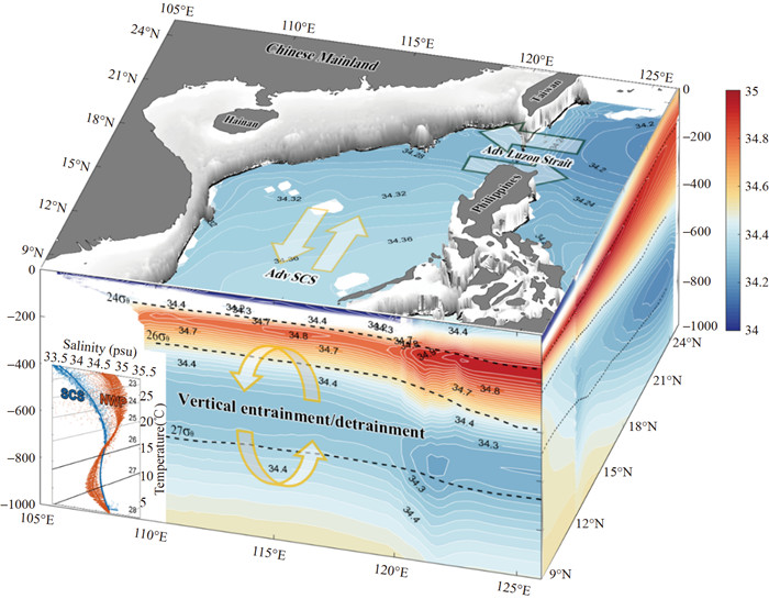
The SCS intermediate water (SCSIW) is located at a depth of 350–800 m, with a potential density of 26–27 kg m^–3 and a salinity range approximately between 34.30–34.50. A minimum salinity layer exists at about 500 m depth with a potential density of 26.8 kg m^–3, which is considered the core of SCSIW (Liu et al. ^[4]; Zhou et al. ^[12]). Liu et al. ^[13] found that the intermediate water of the SCS was freshening between the 1960s and the 1980s. The salinity balance of SCSIW is controlled mainly by the salt advection exchange with the surrounding oceans, as well as the vertical entrainment from both the SCS tropical water and the upper layer of the SCS deep water (Fang et al. ^[14]; Gan et al. ^[15]; Su ^[16]; Xue et al. ^[17]) (Fig. 1). In contrast to that on the currents in the surface and subsurface layers, the intermediate layer salt exchange through the Luzon Strait is still unclear (Qu et al. ^[3]; Tian et al. ^[18]; Liu et al. ^[4]; Zhang et al. ^[19]) due to the lack of research on the water exchange between the north Pacific intermediate water (NPIW) and SCSIW.

Figure 1.  Spatial distribution of the northern South China Sea (NSCS) intermediate layer salinity (units: psu) and schematics of the forcing mechanisms that influence it. The upper plane shows the climatological horizontal distribution of NCSC intermediate salinity and topography shallower than 500 m. The front plane shows the zonal climatological mean salinity in the NSCS (15°N to 22°N); black dash lines indicate isopycnals of 24, 26, and 27σ_θ, which separate the mixing, subsurface, intermediate, and deep layers, respectively. The plane on the right side shows the meridional climatological mean salinity along 125°E. On the lower-left corner are the T-S curves for the NSCS (blue) and northwestern Pacific Ocean (orange).

The long-term variability in intermediate salinity in the NSCS can provide an important indicator for the long-term variation in intermediate circulation in the SCS. However, how the intermediate-layer salinity changes and what drives the change are still not well understood. To answer these questions, this study will investigate the long-term salinity change in the intermediate water in the NSCS using various oceanic dataset products. Through salinity budget analysis, the contribution of horizontal advection as an external force and that of vertical entrainment as an internal dynamic will be studied, and the possible mechanisms of the impacts of thermodynamics processes on the salinity change will be discussed.

The long-term variation in intermediate water salinity in the NSCS was tracked using two oceanic dataset products. The first dataset was obtained from the Institute of Atmospheric Physics (IAP) ocean gridded products supplied by the Chinese Academy of Sciences. The reconstructive monthly IAP dataset is from 1940 to the present, with a resolution of 1° × 1° horizontally and 41 vertical levels ranging from 1–2000 m. The data were primarily input using all of the available measurements (such as Argo, CTD, XBT, bottle, glider) from the World Ocean Database (WOD) (Cheng et al. ^[20]). The IAP product was designed to minimize the sampling errors and is thus particularly suitable for long-term change studies (Cheng et al. ^[21]). The second dataset was obtained from the Ishii products from the Japan Meteorological Agency (JMA), which provided data from 1960 to 2014. This dataset had a horizontal resolution of 1° × 1° and 28 vertical levels ranging from 1–2000 m (Ishii and Kimoto ^[22]).

Data on oceanic currents were used to assess the impacts of horizontal salt transport and vertical entrainment in salinity budget analysis. Horizontal and vertical velocities were obtained from the Simple Ocean Data Assimilation (SODA, version 2.2.4) reanalysis dataset (Carton and Giese ^[23]). Monthly velocity data from SODA has a time coverage from 1960 to 2010, a horizontal resolution of 1/4° × 1/4°, and 40 vertical levels ranging from 1–5000 m.

Salinity budget analysis has been widely used to identify the dynamics processes that mainly contribute to salinity changes. The equation for box-averaged intermediate water salinity budget (Gao et al. ^[24]; Yu ^[25]; Liu et al. ^[26]) is as follows:

where the square brackets denote the depth average within the given layer with potential density between 26–27 kg m^–3 and [S] represents the mean salinity of the intermediate water, $\frac{\partial[S]}{\partial t}$ depicts salinity tendency, h is the intermediate layer depth, defined as the depth at which the potential density is between 26–27 kg m^–3. ∆S is the salinity difference between the intermediate water and upper subsurface water, and the lower top layer in deep water. The variables u, v, and w represent the zonal (x), meridional (y), and vertical (z) velocities, respectively. The subscripts H and Z denote the horizontal and vertical components of the variables, respectively. The first four terms on the right-hand side of Eq. (1) represent horizontal advection, the sum of salt fluxes across the isopycnal due to intermediate layer deepening/shoaling, lateral induction, and vertical advection, respectively. ε represents the residual of the salinity budget, including turbulent diffusion and cross-isopycnal mixing in both the horizontal and vertical directions.

In this study, we consider the intermediate layer in the NSCS (15°–22°N, 108°–120°E) as a box and only consider the salinity exchange through the Luzon Strait (Adv_LZ) and the southern boundary of the NSCS (Adv_SSCS) at 15°N in the horizon. The lateral induction can be ignored because of the few horizontal advections across the gentle-slope top and bottom boundaries of the intermediate layer. The intermediate water salinity budget equation can be simplified as (Zeng et al. ^{[6, 11]}):

where T_in and T_out represent the transports flowing in and out of the NSCS, respectively, T_up and T_bot are the transports across the upper and bottom boundaries of the intermediate layer, respectively. ∆S_WP and ∆S_sscs are the salinity differences between the intermediate water NSCS and the northwest Pacific and southern SCS, respectively, ∆S_sub represents the salinity difference between the intermediate and subsurface layers, and ∆S_deep represents the salinity difference between intermediate and deep layers in the NSCS. Vs is the volume of the NSCS intermediate water. h_up and h_bot are the depth of 26σ_θ and 27σ_θ isohalines where the upper and bottom boundaries of the intermediate layer locate, respectively. H is the thickness of the intermediate layer. The simplified intermediate salinity budget equation contains horizontal advection term (the first term of Eq. (2)), vertical advection term (the second term), deepening/shoaling terms (the third and fourth terms) and ε represents the residual.

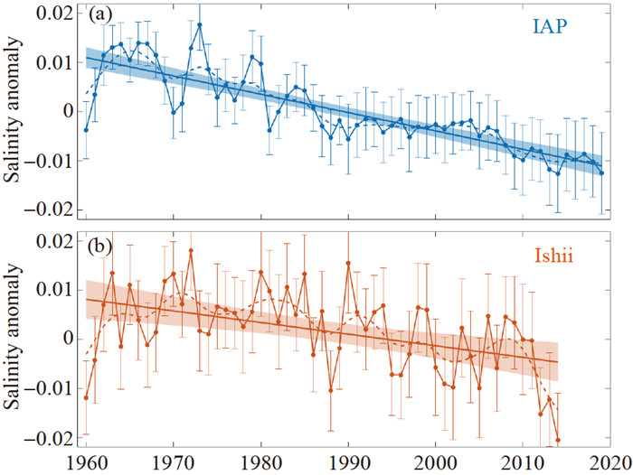
Figure 2 illustrates the time evolution of the averaged salinity of intermediate water in the NSCS. Over the past 60 years, the salinity of intermediate water in the NSCS derived from the IAP dataset has continuously decreased. Notably, the decreasing trend was accompanied by inter-annual variations that were more significant from the 1960s to the 1980s than in subsequent decades. Meanwhile, analysis of the salinity time evolution records from the Ishii dataset also indicated a freshening trend in the intermediate layer over the past few decades, albeit with stronger inter-annual variation than that in the IAP dataset (Fig. 2b). The difference in inter-annual variation could be attributed to the use of distinct reconstruction methods. Despite such differences, there is high consistency between the two datasets regarding the 60-year long-term overall freshening trends, with rates of –0.037 per 100 years in the IAP dataset and –0.024 per 100 years in the Ishii dataset, respectively.

Figure 2.  Time series of the yearly domain averaged intermediate minimum-salinity anomaly based on (a) IAP and (b) Ishii datasets (points and polylines) in the northern South China Sea (NSCS, 15°–22°N, 108°–120°E), with error bars which represent standard deviation, and the low-frequency 7-year filtered values (dash lines). Straight solid lines represent long-term trends, with shaded areas indicating the limits of a 95 percent confidence interval.

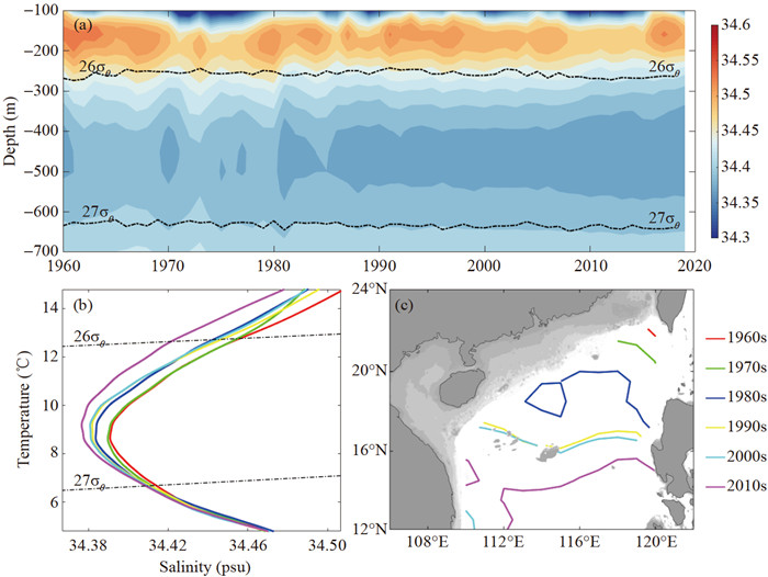
Figure 3a presents the vertical structure of the area-averaged salinity in the NSCS below 100 m over the past 60 years, where the data collected from the IAP dataset was smoothed by using a 7-year moving average to filter out seasonal and inter-annual variation. This clearly reveals a reduction of the salinity in the intermediate layer (between 26σ_θ and 27σ_θ isohalines). The freshening signal was not limited to the core but rather throughout the intermediate layer, indicating a continuous freshening trend based on the IAP dataset in the entire intermediate layer, as shown in Fig. 3b. This suggests that the water mass with lower salinity water mass in the intermediate layer in the NSCS has been moving southward over the past six decades (Fig. 3c).

Figure 3.  (a) Variation in the vertical structure of salinity in the NSCS (15°–22°N, 108°–120°E), smoothed by a 7-year moving average filter. The intermediate layer is located between the two dash lines that represent 26 and 27σ_θ. (b) Decadal mean T-S graphic of the intermediate salinity. Black solid lines represent 26 and 27σ_θ, between which the intermediate layer is located. (c) Locations of decadal mean 34.38 psu isolines; gray shadows indicate the topography shallower than 350 m.

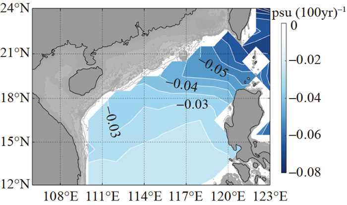
The spatial pattern of the freshening trend of intermediate water salinity in the NSCS is shown in Fig. 4. Generally, there has been a consistent decline in the intermediate water salinity throughout the entire NSCS basin, with linear trends ranging from –0.030 to –0.050 per 100 years depending on locations. The most significant freshening has taken place in the Luzon Strait, which serves as the sole connection between SCSIW and NPIW (You et al. ^[27]). Within this strait, the freshening trend exceeds –0.060 per 100 years, approximately double the mean over the NSCS basin. Additionally, a southwestward freshening-trend gradient has emerged along the northern slope of the NSCS Basin.

Figure 4.  Spatial distribution of the linear freshening trends in the intermediate-layer salinity of NSCS, with gray shadows indicating the topography shallowed than 350m.

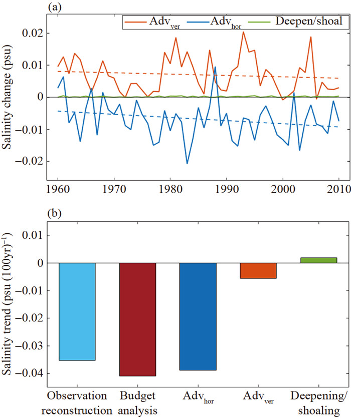
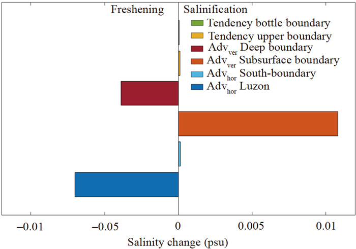
Figure 5a depicts the temporal evolution of the main budget terms in the salinity budget equation (Eq. (2)). The evolution of salinity anomaly in the NSCS intermediate water was mainly controlled by two factors: horizontal advection term (Adv_hor) and vertical advection across the isopycnal (Adv_ver) as part of the vertical entrainment. These two terms played opposite effects on salinity: Adv_hor resulted in a freshwater flux with a positive effect on intermediate freshening, while Adv_ver led to a salt flux with a negative effect. Fig. 6 depicts the contributions of the various dynamics processes to the intermediate salinity change in NSCS. The Adv_hor term was primarily contributed by advection across the Luzon Strait (Adv_LZ), whereas advection across the SSCS boundary (Adv_SSCS) made a much smaller contribution. The Adv_ver term consisted of two opposite-effect advection components. The vertical salinity advection from the subsurface layer (Adv_sub), which was the dominant component of the Adv_ver term, brought more salt flux than the freshwater flux brought by vertical advection from the deep layer (Adv_deep), producing a combined salt flux of the Adv_ver. Compared with the horizontal and vertical advection, the intermediate-layer deepening/shoaling terms, represented by the tendency of isopycnal, had a small and negative contribution to the freshening of the intermediate water in NSCS.

Figure 5.  (a) Temporal evolution (solid polylines) and linear trend (dash straight lines) of the contributions of each term in the salinity budget equation, including horizontal advection term (Adv_hor, blue lines), vertical advection term (Adv_ver, orange lines), and deepening/shoaling term (green line). (b) The first and second bars from the left side represent the linear trend values of the observation reconstruction record (cyan) and budget analysis counting (red). The third to fifth bars are the linear trend values contributed by the horizontal advection term (Adv_hor, blue), vertical advection term (Adv_ver, orange), and deepening/shoaling term (green) in the salinity budget equation, respectively.

Figure 6.  Climatological mean contributions of each term of the salinity budget equation to the intermediate salinity change in the NSCS.

Figure 5a also shows that both Adv_hor and Adv_ver have freshening trends with rates of –0.0389 psu and –0.0056 psu per 100 years, respectively, in which Adv_hor with freshwater flux strengthens and Adv_ver with saltwater flux weakens, favoring the freshening of intermediate water. Fig. 5b illustrates the contributions to the intermediate salinity linear trend from Adv_hor, Adv_ver, and deepening/shoaling terms. The Adv_hor has been the main budget term that affected the intermediate salinity change and made more contribution to the freshening trend than the Adv_ver, which indicated that the horizontal advection through the Luzon Strait mainly affected the intermediate salinity anomaly, whereas vertical advection was the secondary factor. The freshening speed estimated from the salinity budget equation has a value of –0.040 psu per 100 years, close to that recorded in the observed reconstruction data of –0.035 psu per 100 years (the first and second bars in Fig. 5b), which indicates that the result of salinity budget analysis can, by and large, explain the freshening trend of the intermediate salinity and the contributions of dynamics processes in the NSCS.

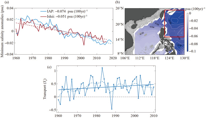
As the only deep-water channel connecting the SCS and the western Pacific, the Luzon Strait plays an essential role in the water-mass characteristics of the NSCS (Qu et al. ^[28]; Tian et al. ^[18]). As the main contributor of freshwater flux, the horizontal salinity advection across the Luzon Strait (Adv_LZ) is influenced by two factors: the salinity long-term trend in the NPIW and the long-term trend of Luzon Strait transport (LST) in the intermediate layer. Previous studies have documented large-scale freshening of the NPIW (Wong et al. ^[29]; Nakanowatari et al. ^[30]) within the northwest Pacific Ocean, which has been one of the most significant freshening regions since the 1950s (Durack et al. ^[31]; Cheng et al. ^[21]). Over the past 60 years, there has been substantial freshening in the area east of the Luzon Strait in the northwest Pacific (14°–25°N, 121°–130°E), which serves as the source area of the SCSIW (Mensah et al. ^[32]). The freshening rate in the West Pacific over the past 60 years was significantly larger than that in the NSCS (Fig. 7a-b). The fresher NPIW flows into the NSCS through the Luzon Strait, resulting in the freshening trend of the NSCSIW to some extent in the past 60 years. The LST plays a significant role in the freshwater flux conveyor of the SCSIW (Qu et al. ^[33]; Wang et al. ^[34]). Westward inflow exists in the Luzon Strait intermediate layer and transports NPIW into SCSIW (Qu et al. ^[3]; Li and Gan ^[35]; Liu et al. ^[4]; You et al. ^[27]; Zhang et al. ^[19]; Zhou et al. ^[12]). There has been an intensification in the westward intermediate LST over the past decades (Fig. 7c). This has resulted in more freshwater flux into NSCS and further contributed to the freshening of SCSIW. The strengthening of intermediate LST, combined with the freshening of NPIW, transported more low-salinity water into the NSCS as well as the southward freshwater flux, resulting in the freshening trend of SCSIW.

Figure 7.  (a) Time series of the domain averaged salinity anomaly in the northwest Pacific [red box in (b)] intermediate layer. (b) Linear trends in the northwest Pacific intermediate water freshening velocity. (c) Time series (polyline) and trend (straight line) in the Luzon Strait intermediate-layer transport (positive indicates westward) from SODA2.2.4 dataset.

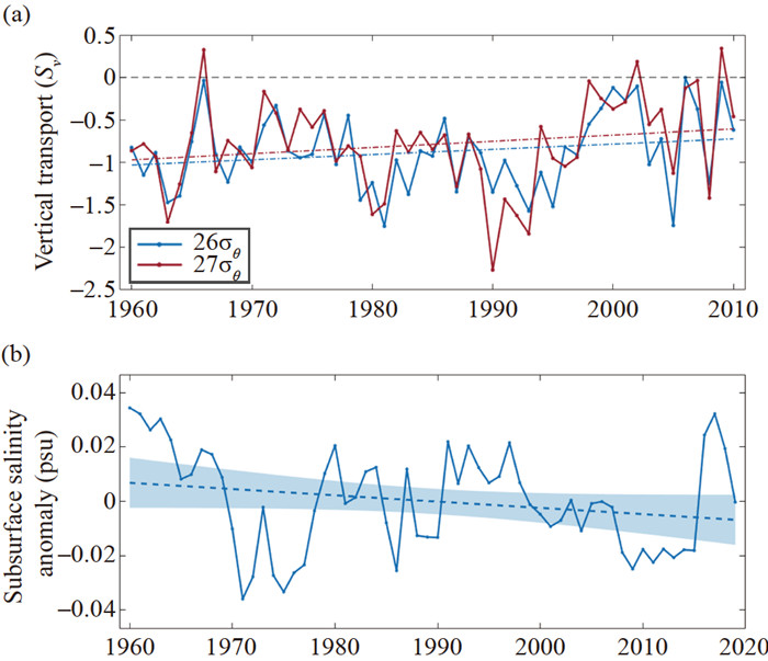
The horizontal layer spinning circulation and unique topography induce complex vertical dynamics in the NSCS (Cai and Gan ^[36]; Chao et al. ^[37]; Gan et al. ^[38]; Lan et al. ^[39]), which can also affect the intermediate salinity by vertical-advection processes as the main contribution of the high-salinity flux in the budget analysis. There is an overall downwelling in the NSCS (Shu et al. ^[40]; Zhu et al. ^[41]), influencing the salinity change in SCSIW by bringing high salt flux into and freshwater flux out of the intermediate layer. As the downwelling across the intermediate layer has slowed down in the past decades (Fig. 8a), the high-salinity flux transport from the subsurface layer, where the saltiest South China Sea tropical water is located, has weakened and resulted in a decreasing trend of high-salinity vertical entrainment. In the boundary of the intermediate layer and deep layer, the freshwater flux has also decreased so that more fresh water remains, keeping the freshening trend in SCSIW. Generally, the decreasing vertical entrainment, accompanied by the freshening of the upper-layer water (Nan et al. ^[42]) (Fig. 8b), becomes the secondary factor affecting the long-term freshening of SCSIW. Moreover, the SCS meridional overturning circulation showed a weakening trend over the past 60 years (Yang and Luo ^[43]), with the slowdown of the vertical exchange (Zhu et al. ^{[44, 45]}), which in turn affects the exchange between the intermediate and deep layers, and contributes to the decreasing trend of vertical salinity transport.

Figure 8.  (a) Time series and trends of the annual mean domain averaged vertical transport across 26σ_θ and 27σ_θ isohalines in the NSCS. (b) Variations and trends of the annual mean spatial average subsurface-layer salinity anomaly in the NSCS, with shaded areas indicating the limits of 95 percent confidence interval.

In this study, we have identified a 60-year freshening trend in salinity in the intermediate layer of the NSCS, with a freshening velocity of approximately –0.037 per 100 years in the IAP reconstructive data. Through salinity budget analysis, we investigated various dynamical factors that contribute to the intermediate salinity trend in the NSCS. The results reveal that horizontal advection, driven by the LST, and vertical entrainment from the subsurface layer are significant drivers of this long-term variability. The primary reason for the freshening of intermediate water in the NSCS is the influx of more freshwater flux, which comes from the strengthening of intermediate LST and a quicker freshening rate in NPIW. Additionally, the freshening of the SCS tropical water and the slowdown of the vertical movement might also contribute to the freshening of the intermediate water in the NSCS by reducing the salt flux through vertical entrainment. As the response to the change of the regional oceanic dynamic processes, the freshening of the intermediate water in the NSCS will affect not only the thermodynamic and dynamic environment in nearby regions such as the southern SCS but also the salinity in the subsurface and deep water in NSCS. The reaction between the change of salinity and the variation of dynamic processes is still waiting for further research.

It should be noted that there are some uncertainties in this study. The use of different datasets to calculate different terms in salinity budget analysis might lead to a certain level of dynamical inconsistency. Furthermore, the data uncertainty in each dataset is poorly known, especially in the intermediate SCS, where observations are not abundant. This uncertainty is mainly associated with the sampling, thus potentially leading to a common error in all of the datasets, which rely on essentially the same in situ dataset (i.e., WOD). With the increasing number of available observations in the future, more quantitative research will be needed.